One Ciphertext, Many Messages: SIMD operations in FHE

Fully Homomorphic Encryption (FHE) promises a revolutionary capability: performing arbitrary computations on encrypted data without ever decrypting it. This breakthrough enables secure cloud computing where sensitive data remains protected even during processing. However, early FHE schemes faced a critical bottleneck. Consider a simple task like adding two encrypted vectors of length 1000. This would require 1000 separate homomorphic additions, each involving expensive operations on large polynomials. For real-world applications processing massive datasets, this element-by-element approach creates prohibitive computational overhead.

Modern FHE schemes like BGV, BFV and CKKS solve this challenge through an elegant mathematical insight: they can pack multiple plaintext values into a single ciphertext and perform operations on all packed values simultaneously.

Instead of encrypting individual numbers, these schemes:

• Pack hundreds or thousands of values into "slots" within a single ciphertext
• Perform homomorphic operations that affect all slots in parallel
• Support sophisticated data movement operations like rotations and permutations

This Single Instruction, Multiple Data (SIMD) approach transforms FHE from a theoretical curiosity into a practical tool. A single homomorphic multiplication can now process an entire vector at once, delivering speedups of several orders of magnitude.

This post explores the mathematical foundations underlying these SIMD operations. We'll see how abstract concepts from algebra and number theory combine to create a powerful framework for parallel homomorphic computation. While the mathematics is sophisticated, understanding these foundations is crucial for implementing efficient FHE applications and pushing the boundaries of what's possible with encrypted computation.

Mathematical Foundations

This post assumes you're comfortable with the basics of groups and rings, things like the distributive laws and fundamental properties of rings with identity. If you've worked with elementary group theory, you should be in good shape.

Ideals

Definition. Let $R$ be a ring. A subset $I \subseteq R$ is called an ideal when:

1. $(I, +)$ forms a subgroup of $(R, +)$
2. For any $r \in R$ and $a \in I$, both $r \times a$ and $a \times r$ belong to $I$

That second condition is what makes ideals special, they "absorb" multiplication by any element in the ring. It's like having a mathematical black hole that pulls in anything you multiply with it.

Example. In the integers $\mathbb{Z}$, consider the set $n\mathbb{Z} = \{nk \mid k \in \mathbb{Z}\}$ of all multiples of $n$. This forms an ideal because multiplying any multiple of $n$ by any integer gives you another multiple of $n$.

Principal Ideals

A principal ideal is the simplest kind, one generated by a single element. Given $a \in R$, we can create the ideal

$$(a) = \{r \times a \mid r \in R\}.$$

This captures the smallest ideal that contains $a$. It's everything you can get by multiplying $a$ by elements from the ring.

Building New Rings: Quotients

Given a ring $R$ and an ideal $I$, we can construct a brand new ring called the quotient ring $R/I$.

The elements of $R/I$ are cosets, think of them as equivalence classes $a + I = \{a + i \mid i \in I\}$ for $a \in R$. We define operations on these cosets by:

• Addition: $(a + I) + (b + I) = (a + b) + I$
• Multiplication: $(a + I) \times (b + I) = (a \times b) + I$

Examples:

1. $\mathbb{Z}/n\mathbb{Z}$: This gives us the familiar "clock arithmetic" - integers modulo $n$ with elements $\{0, 1, 2, \ldots, n-1\}$.

2. Polynomial quotients: Taking $R = \mathbb{F}[X]$ and $I = (f(X))$, we get polynomials modulo $f(X)$ - essentially polynomial arithmetic where we replace high powers using the relation $f(X) = 0$.

Roots of Unity

In any ring $R$, an $n$-th root of unity is an element $\zeta$ such that $\zeta^n = 1$. But we're particularly interested in primitive $n$-th roots of unity $\zeta^k \neq 1$ for all positive integers $k < n$.

Here's a key insight: $\zeta_n^k$ is a primitive $n$-th root of unity if and only if $\gcd(k,n)=1$.

Why this works

Let $\zeta_n = e^{2\pi i / n}$. The $n$-th roots of unity are the $n$ distinct powers $\zeta_n^0, \zeta_n^1, \ldots, \zeta_n^{n-1}$, so $\zeta_n$ itself is primitive.

The key observation is that $\zeta_n^a = 1$ if and only if $a$ is divisible by $n$. Here's why: write $n = aq + r$ with $0 \leq r < a$. Then $\zeta_n^r = \zeta_n^{n-aq} = 1$. But since $\zeta_n$ is primitive, this only happens when $r = 0$.

Now, if $\gcd(k,n) = d > 1$, then $(\zeta_n^k)^{n/d} = \zeta_n^{k \cdot n/d} = \zeta_n^{n \cdot k/d} = 1$, so $\zeta_n^k$ is not primitive.

Conversely, if $\gcd(k,n) = 1$ and $(\zeta_n^k)^r = 1$, then $n$ divides $kr$. Since $n$ and $k$ are coprime, we must have $n$ divides $r$. This means the first positive power of $\zeta_n^k$ that equals $1$ is the $n$-th power.

Euler's totient function $\varphi(n)$ counts exactly these "good" exponents - the positive integers $k \leq n$ that are coprime to $n$. So there are precisely $\varphi(n)$ primitive $n$-th roots of unity.

Example. In the complex numbers, the primitive $n$-th roots of unity are exactly $e^{2\pi i k/n}$ where $\gcd(k,n) = 1$.

Euler's totient function $\varphi(n)$ counts the positive integers up to $n$ that are coprime to $n$: $\varphi(n) = |\{1 \leq k \leq n \mid \gcd(k,n)=1\}|$

A Concrete Example: 8th Roots of Unity in $\mathbb{F}_{3^2}$

Let's work out a specific case. We'll find the 8th roots of unity in the quadratic extension

$$\mathbb{F}_{3^2} = \mathbb{F}_3[X]/(X^2+1)$$

How Many Roots Should We Expect?

In a finite field of size $q$, the multiplicative group $\mathbb{F}_q^{\times}$ has order $q-1$.

• If $n$ is coprime to $q-1$, then $\mathbb{F}_q$ contains only the trivial $n$-th root of unity: just $1$.
• If $n$ divides $q-1$, the field contains exactly $n$ distinct $n$-th roots of unity, forming the unique subgroup of that order.

Here, $q = 9$, so $q-1 = 8$. Since $8$ divides $8$, we expect all eight 8th roots of unity to live inside $\mathbb{F}_{3^2}^{\times}$.

Finding All Eight Roots

We write elements of $\mathbb{F}_{3^2}$ in the form $a+bx$ with $a,b \in \{0,1,2\}$, where $x^2 = -1 \equiv 2 \pmod{3}$.

Using Sage (or by hand if you're feeling ambitious):

R.<t> = PolynomialRing(GF(3))          
F.<x> = GF(3^2, modulus = t^2 + 1) 

roots8 = [z for z in F if z^8 == 1]     
print(roots8)

This gives us:

$$1, x + 1, 2x, 2x + 1, 2, 2x + 2, x, x + 2$$

All eight solutions to $z^8 = 1$ in $\mathbb{F}_{3^2}$.

Which Ones Are Primitive?

An element is primitive when its order is exactly $8$. Euler's totient tells us $\varphi(8) = 4$, so exactly four of our eight roots should be primitive.

g = F.multiplicative_generator() 
primitive = [g^k for k in (1,3,5,7)]   
print(primitive)

This reveals:

$$\{x+1, 2x+1, 2x+2, x+2\}$$

These are our four primitive 8th roots. The remaining roots have orders 1, 2, or 4.

Cyclotomic Polynomials: Collecting the Primitives

The $n$-th cyclotomic polynomial $\Phi_n(X)$ is designed to capture exactly the primitive $n$-th roots of unity. Over the rationals:

$$\Phi_n(X) = \prod_{\substack{1 \leq k \leq n\\\gcd(k,n)=1}} (X - \zeta_n^k)$$

This polynomial has degree $\varphi(n)$ - one factor for each primitive root.

Let's construct $\Phi_8(X)$

By definition:

$$\Phi_8(X) = \prod_{\substack{1 \leq k \leq 8\\\gcd(k,8)=1}} (X-\zeta_8^k) = X^4+1$$

This gives us a monic quartic (degree $\varphi(8) = 4$) that's irreducible over $\mathbb{Q}$.

Homomorphisms: Structure-Preserving Maps

Group Homomorphisms

A group homomorphism between groups $(G, \cdot)$ and $(H, *)$ is a function $\phi: G \to H$ that respects the group operation:

$$\phi(a \cdot b) = \phi(a) * \phi(b)$$

Two important subsets come with every homomorphism:

• The kernel: $\ker(\phi) = \{g \in G \mid \phi(g) = e_H\}$ (elements that map to the identity)
• The image: $\text{im}(\phi) = \{\phi(g) \mid g \in G\}$ (all possible outputs)

Both form subgroups of their respective groups.

Ring Homomorphisms

Similarly, a ring homomorphism between rings $(R, +, \times)$ and $(S, \oplus, \odot)$ preserves both operations:

• $\psi(a + b) = \psi(a) \oplus \psi(b)$
• $\psi(a \times b) = \psi(a) \odot \psi(b)$
• $\psi(1_R) = 1_S$ (preserves multiplicative identity)

Isomorphisms: When Structures Are "The Same"

When a homomorphism is bijective, we call it an isomorphism. Isomorphic structures are essentially identical from an algebraic perspective - they have the same "shape."

An automorphism is an isomorphism from a structure to itself. The collection of all automorphisms of a group $G$ forms a group under composition, denoted $\text{Aut}(G)$.

The Chinese Remainder Theorem: A Powerful Decomposition

Let $R$ be a commutative ring with unity, and let $I_1, I_2, \ldots, I_n$ be comaximal ideals (meaning $I_i + I_j = R$ whenever $i \neq j$). Define $I = I_1 \cap I_2 \cap \cdots \cap I_n$. Then we have an isomorphism:

$$R/I \cong (R/I_1) \times (R/I_2) \times \cdots \times (R/I_n)$$

Why this works

We'll prove this by induction on the number of ideals.

Base Case ($n = 2$): Let $I, J$ be comaximal ideals with $I + J = R$. We want to show $R/(I \cap J) \cong (R/I) \times (R/J)$.

Consider the natural map:

$$\varphi: R \to (R/I) \times (R/J), \quad x \mapsto (x+I, x+J)$$

By the First Isomorphism Theorem, it suffices to show $\varphi$ is surjective with kernel $I \cap J$.

First Isomorphism Theorem for Rings: If $\varphi\colon R \;\longrightarrow\; S$ is a surjective ring homomorphism with kernel $\ker(\varphi)$, then $\varphi$ induces a natural ring isomorphism

$$\varphi: R/\ker(\varphi) \;\xrightarrow{\;\sim\;}\; S, \qquad r + \ker(\varphi)\mapsto\;\varphi(r).$$

Kernel verification: We have

$$x \in \ker\varphi \Leftrightarrow (x+I, x+J) = (0+I, 0+J) \Leftrightarrow x \in I \text{ and } x \in J \Leftrightarrow x \in I \cap J$$

Surjectivity: Take any $(x_1+I, x_2+J) \in (R/I) \times (R/J)$. Since $I + J = R$, we can find $y_1 \in I$ and $y_2 \in J$ with $y_1 + y_2 = 1$.

Define $x = x_1 + y_1(x_2 - x_1) = x_2 - y_2(x_2 - x_1)$.

Then $x \equiv x_1 \pmod{I}$ and $x \equiv x_2 \pmod{J}$, so $\varphi(x) = (x_1+I, x_2+J)$.

Inductive Step: Suppose the theorem holds for $n$ ideals. For $n+1$ comaximal ideals $I_1, \ldots, I_{n+1}$, observe that $I_1, \ldots, I_{n-1}, I_n \cap I_{n+1}$ are pairwise comaximal.

By the inductive hypothesis:

$$R/I \cong (R/I_1) \times \cdots \times (R/I_{n-1}) \times (R/(I_n \cap I_{n+1}))$$

Applying the base case to $I_n$ and $I_{n+1}$:

$$R/(I_n \cap I_{n+1}) \cong R/I_n \times R/I_{n+1}$$

Combining these gives the desired result.

SIMD Operations in Fully Homomorphic Encryption

Now we get to the exciting part - how all this abstract algebra enables powerful parallel computation in encrypted data.

Where Our Polynomials Live

We start with a quotient ring $A = \mathbb{Z}[X]/(\Phi_m(X))$, where $\Phi_m(X)$ is the $m$-th cyclotomic polynomial. This is our fundamental workspace.

In homomorphic encryption, we don't encrypt integers directly. Instead, we work over a prime field $\mathbb{F}_p = \mathbb{Z}/p\mathbb{Z}$ that serves as our plaintext space. Reducing all coefficients modulo $p$ gives us the plaintext ring:

$$A_p = \mathbb{F}_p[X]/(\overline{\Phi_m}(X))$$

The overline just reminds us we've done the modular reduction.

The Magic of Cyclotomic Factorization

Here's where number theory delivers something beautiful. As long as $p$ doesn't divide $m$, the cyclotomic polynomial $\Phi_m(X)$ completely factors over $\mathbb{F}_p$ into irreducible pieces of equal degree:

$$\overline{\Phi_m}(X) = F_1(X) F_2(X) \cdots F_n(X) \bmod p$$

Each $F_i$ is irreducible with degree $d = \text{ord}_m(p)$ - the multiplicative order of $p$ modulo $m$.

Let's pick any irreducible factor, say $F_1(X)$, and define:

$$E = \mathbb{Z}_p[X]/(F_1(X)), \quad \eta = [X \bmod F_1(X)] \in E$$

Since $F_1(X)$ is irreducible, $E$ becomes a field with $p^d$ elements. Every element in $E$ can be written as $f(\eta)$ for some polynomial $f(X)$. Notice that $\eta$ is a root of $F_1(X)$, making it a primitive $m$-th root of unity.

Why the coset $\eta=[X]$ is instantly a root of $F_1$: Forming the quotient ring
$E = \mathbb{Z}_p[X]/(F_1(X))$
is nothing more than declaring inside the ring that the polynomial $F_1(X)$ now equals zero.

• The projection $\pi:\mathbb{Z}_p[X]\to E$ sends every polynomial to its coset. Write
  $\eta := \pi(X) = X + (F_1(X)).$
  This $\eta$ is the “image of $X$’’.
• Because $F_1(X)$ is in the ideal we factor by, its coset is $0$: $\pi\bigl(F_1(X)\bigr)=0.$
  But $\pi$ is a homomorphism, so $\pi\bigl(F_1(X)\bigr)=F_1\bigl(\pi(X)\bigr)=F_1(\eta)$. Hence $F_1(\eta)=0$ in $E$. By construction, $\eta$ behaves exactly like a root of $F_1$.

The polynomial $\overline{\Phi_m}(X)$ has $\varphi(m)$ distinct roots in $E$, specifically $\eta^j$ for each $j$ in the unit group $\mathbb{Z}_m^*$. These roots distribute evenly among the irreducible factors, with each factor getting exactly $d$ roots.

To understand the distribution, consider the subgroup:

$$H = \langle \bar{p} \rangle \subset \mathbb{Z}_m^*, \quad \bar{p} := [p \bmod m]$$

This subgroup has order $d$ and contains $1, \bar{p}, \bar{p}^2, \ldots, \bar{p}^{d-1}$.

When we form the quotient group $\mathbb{Z}_m^*/H$, we get $n = \varphi(m)/d$ distinct cosets:

$$kH = \{k \cdot h : h \in H\} \subset \mathbb{Z}_m^*$$

Choosing representatives $k_1, k_2, \ldots, k_n$ from each coset, we can arrange things so each $F_i(X)$ has exactly the $d$ roots $\eta^k$ where $k \in k_i H$.

The Chinese Remainder Breakthrough

Now comes the payoff. We can establish isomorphisms for each factor:

$$\mathbb{Z}_p[X]/(F_i(X)) \to E, \quad [f(X) \bmod F_i(X)] \mapsto f(\eta^{k_i})$$

Combining this with the fact that

$$\begin{array}{rcl} A_{p} & \longrightarrow & \displaystyle \Bbb Z_{p}[X]\bigl/\!\bigl(F_{1}(X)\bigr) \;\times\; \cdots \;\times\; \Bbb Z_{p}[X]\bigl/\!\bigl(F_{n}(X)\bigr) \\[6pt] f(x) & \longmapsto & \bigl(\, [\,f(X)\bmod F_{1}(X)\,],\; \ldots,\; [\,f(X)\bmod F_{n}(X)\,] \bigr), \end{array}$$

gives us the crucial isomorphism:

$$A_p \to E^n, \quad f(x) \mapsto (f(\eta^{k_1}), \ldots, f(\eta^{k_n}))$$

This is the key insight: we can perform component-wise operations on vectors in $E^n$ by doing ring operations in $A_p$!

If we have:

$$\begin{gathered} a \in A_p \leftrightarrow (\alpha_1, \ldots, \alpha_n) \in E^n \\ b \in A_p \leftrightarrow (\beta_1, \ldots, \beta_n) \in E^n \end{gathered}$$

Then:

$$\begin{gathered} a + b \leftrightarrow (\alpha_1 + \beta_1, \ldots, \alpha_n + \beta_n) \\ a \cdot b \leftrightarrow (\alpha_1\beta_1, \ldots, \alpha_n\beta_n) \end{gathered}$$

Converting between the coefficient representation in $A_p$ and the slot representation in $E^n$ is computationally straightforward using the Number Theoretic Transform (NTT).

Cyclotomic Polynomial Example: NTT Implementation

Let's work through a concrete example with specific parameters:

• $m = 8$, $\varphi(m) = 4$, $p = 3$, $d = 2$ (since $3^2 \equiv 1 \bmod 8$), $n = \varphi(m)/d = 2$

Cyclotomic Polynomial Factorization

The 8th cyclotomic polynomial is $\Phi_8(X) = X^4 + 1$. Over $\mathbb{F}_3[X]$, this splits as:

R.<X> = PolynomialRing(GF(3))
factor = (X^4 + 1).factor()
print(factor)      

$$X^4 + 1 = (X^2 + X + 2)(X^2 + 2X + 2) \quad \text{in } \mathbb{F}_3[X]$$

The four primitive 8th roots of unity are:

$$\{\alpha+1, 2\alpha+1, 2\alpha+2, \alpha+2\} \subset E$$

Each irreducible quadratic "owns" exactly two of them:

Polynomial	Roots in $E$
$X^2 + X + 2$	$\{2\alpha+1, \alpha+1\}$
$X^2 + 2X + 2$	$\{2\alpha+2, \alpha+2\}$

Cosets and the Chinese Remainder Theorem Isomorphism

The coset structure is determined by:

• Subgroup: $H = \langle 3 \rangle = \{1, 3\} \subset \mathbb{Z}_8^*$
• Quotient: $\mathbb{Z}_8^*/H = \{\{1,3\}, \{5,7\}\}$
• Representatives: $k_1 = 1$, $k_2 = 5$

This gives us the isomorphism:

$$A_3 = \mathbb{F}_3[X]/(X^4+1) \xrightarrow{\sim} E^2$$ $$f(x) \mapsto (f(\eta^{k_1}), f(\eta^{k_2})) = (f(\alpha+1), f(2\alpha+2))$$

Inverse Transform: Slot Values to Polynomial

We want to encode the following slot values:

$$f(\eta)=2,\qquad f\!\bigl(\eta^5\bigr)=1,$$

where $\eta = \alpha+1$.

Polynomial Representation

Any polynomial in $A_3$ has a unique representative:

$$f(X)=a_0+a_1X+a_2X^{2}+a_3X^{3},\qquad a_i\in\mathbf F_{3}.$$

This means we need 4 evaluations of our function to interpolate it using NTT. Because the Frobenius automorphism $x \mapsto x^{3}$ fixes each $\Bbb F_{3}$ component, we have:

$$f(\eta)= 2 = f(\eta^{3}),\qquad f(\eta^{5})= 1 = f(\eta^{7})$$

Setting Up the Inverse NTT

Indeed
$\omega:=\eta^{2}=2x$, $\omega^{2}=(2x)^{2}=4x^{2}=x^{2}=2$,
$\omega^{4}=2^{2}=1$,
and $\omega\neq1$, $\omega^{2}\neq1$, so $\omega$ is a primitive $4$-th root of unity.

We need $f$ evaluated at the odd powers of $\eta$:

$$\{\,\eta^{1},\eta^{3},\eta^{5},\eta^{7}\} =\{\,\eta\,\omega^{0},\,\eta\,\omega^{1},\,\eta\,\omega^{2},\,\eta\,\omega^{3}\}.$$

Factor out $w^{j}$ and absorb it into the coefficients:

$$\begin{aligned} f\!\bigl(w^{2k+1}\bigr) &=\sum_{j=0}^{3} a_{j}\bigl(w^{2k+1}\bigr)^{j}\\[4pt] &=\sum_{j=0}^{3} a_{j}\,w^{j}\,(\omega^{k})^{j} \;=\; \sum_{j=0}^{3} b_{j}\,\omega^{jk}, \end{aligned}$$

Thus

• Twist $b=D_{\text{in}}\,a$ where $D_{\text{in}}=\operatorname{diag}(1,w,w^{2},w^{3})$.
• NTT $y=F\,b$ with $F_{k,j}=\omega^{jk}$.

Untwisting after the inverse NTT

Inverse NTT returns $b=F^{-1}y$. Remove the twist:

$$\,a_{j}=b_{j}\,w^{-j}=b_{j}\,w^{8-j}\,$$

All coefficients are now back in $\mathbb{F}_{3}$.

Thus:

$$f(X)=a_{0}+a_{1}X+a_{2}X^{2}+a_{3}X^{3}=X^{3}+X,$$

Sanity Check

We can verify that the polynomial obtained is correct by checking the slot values:

• Slot 0: $f(X) \mod (X^2 + X + 2) = 2$
• Slot 1: $f(X) \mod (X^2 + 2X + 2)= 1$

Everything matches the given slot values, confirming that the reconstruction is correct.

Adding the second polynomial

Let's do the same transformation for the case

$$f(\eta)=x+2,\qquad f\!\bigl(\eta^5\bigr)=2x,$$

First we find the missing evaluations

$$f(\eta^{3}) = f(\eta)^3 = 2 + 2x,\qquad f(\eta^{7}) = f(\eta^5)^3 = x$$

Then going through the same inverse NTT process we get

$$f(X)=X + 1$$

Homomorphic addition

We have

$$X^3 + X \mapsto (2, 1), \qquad X + 1 \mapsto (x+2, 2x)$$

Let’s check that homomorphic addition is well-defined:

$$X^3 + 2X + 1 \mapsto (x+1, 2x+1)$$

Finding the missing evaluations:

$$f(\eta^{3}) = f(\eta)^3 = 1 + 2x,\qquad f(\eta^{7}) = f(\eta^5)^3 = 1 + x$$

and running inverse NTT to reconstruct the polynomial

$$f(X)=X^3 + 2X + 1$$

F3  = GF(3)
F9.<x> = GF(9, modulus = x^2 + 1)   
R.<X> = PolynomialRing(F3)

slot0, slot1 = (2, 1)
           
w   = x + 1                            
omega = w^2                            
omega_inv = omega.inverse()            

y0, y2 = F9(slot0), F9(slot1)
y1, y3 = y0^3, y2^3
y      = [y0, y1, y2, y3]              

b = []
for j in range(4):
    s = F9.zero()
    for k in range(4):
        s += y[k] * (omega_inv)^(j*k)  
    b.append(s)
    
a = [F3(b[j] * w^(8 - j))  for j in range(4)]   


f = (a[0] + a[1]*X + a[2]*X^2 + a[3]*X^3) % (X^4 + 1)

print(f)

Galois Automorphisms: The Key to Data Movement

To understand how to move data between slots, we return to our ring $A = \mathbb{Z}[X]/(\Phi_m(X))$, with $x$ representing the image of $X$ in $A$.

For each $j \in \mathbb{Z}_m^*$, we can define:

$$\theta_j : A \to A, \quad \theta_j(f(x)) = f(x^j)$$

This is well-defined because if $\gcd(j,m) = 1$, then whenever $\omega$ is a primitive $m$-th root of unity, so is $\omega^j$. This means that if $\Phi_m(\omega) = 0$, then $\Phi_m(\omega^j) = 0$ as well, giving us:

$$\Phi_m(X) \mid \Phi_m(X^j) \quad \text{in } \mathbb{Z}[X]$$

These maps have a natural group structure: since $(x^j)^k = x^{jk}$ in $A$, we have:

$$\theta_j \circ \theta_k = \theta_{jk}$$

This gives us an injective group homomorphism:

$$\mathbb{Z}_m^* \hookrightarrow \text{Aut}(A), \quad j \mapsto \theta_j$$

These $\theta_j$ maps are precisely the Galois automorphisms of our cyclotomic extension.

The Frobenius Map: A Special Automorphism

The Frobenius automorphism deserves special attention:

$$\sigma : E \to E, \quad f(\eta) \mapsto f(\eta^p)$$

For every $\alpha \in E$, we have $\sigma(\alpha) = \alpha^p$. Importantly:

$$\alpha \in \mathbb{Z}_p \Leftrightarrow \sigma(\alpha) = \alpha$$

Under our correspondence between $A_p$ and $E^n$, if we let $\bar{p} = [p \bmod m] \in \mathbb{Z}_m^*$ and apply $\theta_{\bar{p}}$:

$$\theta_{\bar{p}}(f(x)) \to(\sigma(f(\eta^{k_1})), \ldots, \sigma(f(\eta^{k_n}))) \in E^n$$

This means $\theta_{\bar{p}}$ acts slot-wise as the Frobenius map on $E$ - crucial for understanding rotations.

One-Dimensional Rotations: Making Data Move

Consider an element $g \in \mathbb{Z}_m^*$ such that $1, g, g^2, \ldots, g^{n-1}$ forms a complete set of coset representatives for $H$ in $\mathbb{Z}_m^*$. This means $g^n$ must lie in $H$.

In the ideal case where $g^n = 1$, using representatives $1, g, \ldots, g^{n-1}$, our slot isomorphism becomes:

$$f(x) \in A_p \leftrightarrow (f(\eta^1), f(\eta^g), \ldots, f(\eta^{g^{n-1}})) \in E^n$$

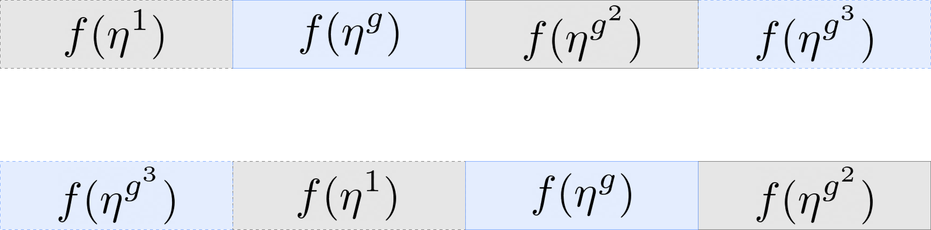
When we apply $\theta_g$:

$$\theta_g(f(x)) \leftrightarrow (f(\eta^g), f(\eta^{g^2}), \ldots, f(\eta^{g^{n-1}}), f(\eta^1))$$

Since the last entry wraps around to $f(\eta^1)$, the automorphism $\theta_g$ rotates the slots one position to the left! More generally, $\theta_{g^e}$ rotates left by $e$ positions, while $\theta_{g^{-e}}$ rotates right by $e$ positions.

When $g^n \neq 1$, things get trickier. If $g^n = \bar{p}^s$ for some $s \in \{1, \ldots, d-1\}$:

$$\theta_g(f(x)) \leftrightarrow (f(\eta^g), f(\eta^{g^2}), \ldots, f(\eta^{g^{n-1}}), \sigma^s(f(\eta^1)))$$

This gives a rotation, but the last slot gets perturbed by $\sigma^s$. This isn't a clean rotation unless the first slot contains a value in $\mathbb{Z}_p$, where $\sigma^s$ acts trivially.

Clean Rotations Through Masking

Even when slots contain values outside $\mathbb{Z}_p$, we can achieve perfect rotations using a clever masking technique.

For a rotation by $e \in \{1, \ldots, n-1\}$ positions, we create masking elements:

$$M_e \in A_p \leftrightarrow (\underbrace{1,\ldots,1}_{n-e}, \underbrace{0,\ldots,0}_{e}) \in E^n$$ $$1-M_e \in A_p \leftrightarrow (\underbrace{0,\ldots,0}_{n-e}, \underbrace{1,\ldots,1}_{e}) \in E^n$$

For an element $a \in A_p \leftrightarrow (\alpha_0, \ldots, \alpha_{n-1}) \in E^n$:

• Mask-then-rotate left by $e$ slots:

$$M_e \cdot \theta_{g^e}(a) \leftrightarrow (\alpha_e, \ldots, \alpha_{n-1}, \underbrace{0,\ldots,0}_{e})$$

• Mask-then-rotate right by $e$ slots:

$$(1-M_e) \cdot \theta_{g^{e-n}}(a) \leftrightarrow (\underbrace{0,\ldots,0}_{n-e}, \alpha_0, \ldots, \alpha_{e-1})$$

Combining these gives a perfect left rotation:

$$M_e \cdot \theta_{g^e}(a) + (1-M_e) \cdot \theta_{g^{e-n}}(a)$$

This produces an element whose slots are exactly those of $a$ rotated $e$ places to the left, regardless of whether slot values lie outside $\mathbb{Z}_p$.

Multi-Dimensional Operations: The Hypercube Approach

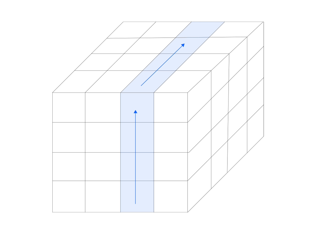
For more complex data arrangements, we can organize our $n$ slots as a multi-dimensional hypercube. Let $n = n_1 n_2 \cdots n_\ell$ be our slot count factored into $\ell$ positive integers.

We choose generators $g_1,\dots,g_\ell\;\in\;\mathbb{Z}_m^{*}$ and arrange the coset representatives as:

$$g_1^{\,e_1}\,g_2^{\,e_2}\cdots g_\ell^{\,e_\ell}, \qquad e_i\in[n_i]:=\{0,\dots,n_i-1\}$$

This creates an $\ell$-dimensional hypercube with side-lengths $(n_1,\dots,n_\ell)$, where every slot has coordinates $(e_1,\dots,e_\ell)$.

Axis-wise Rotations Made Simple

For each dimension $i$, the Galois automorphism $\theta_{g_i}$ shifts every hyper-column $(e_1,\dots,e_{i-1},*,e_{i+1},\dots,e_\ell)$ forward by one step in the $i$-th coordinate. Applying $\theta_{g_i^{\,e}}$ shifts by $e$ positions, while $\theta_{g_i^{-e}}$ shifts backwards.

Multi-Dimensional Masking

For true rotations without Frobenius disturbance, we use masking elements $M^{(i)}_{e}$ that place ones in the first $n_i-e$ slots of each hyper-column and zeros elsewhere.

The formula for rotating left by $e$ positions along the $i$-th axis is:

$$M^{(i)}_{e}\,\theta_{g_i^{\,e}}(a)\;+\;(1-M^{(i)}_{e})\,\theta_{g_i^{\,e-n_i}}(a)$$

SIMD Operations in BGV with Lattigo

This example demonstrates slot-wise homomorphic addition using the Lattigo library’s BGV API. With BGV’s powerful SIMD capabilities, we can pack an entire vector of integers into a single ciphertext, perform encrypted computations on each vector entry in parallel, and then recover the results after decryption.

package main

import (
    "fmt"
    "log"
    "math/rand"
    "time"

    "github.com/tuneinsight/lattigo/v6/examples"
    "github.com/tuneinsight/lattigo/v6/schemes/bgv"
)

func main() {
    paramDef := examples.BGVParamsN12QP109
    params, err := bgv.NewParametersFromLiteral(paramDef)
    if err != nil {
        log.Fatalf("params error: %v", err)
    }

    kgen := bgv.NewKeyGenerator(params)
    sk := kgen.GenSecretKeyNew()
    pk := kgen.GenPublicKeyNew(sk)

    encoder := bgv.NewEncoder(params)
    encryptor := bgv.NewEncryptor(params, pk)
    decryptor := bgv.NewDecryptor(params, sk)
    evaluator := bgv.NewEvaluator(params, nil)

    T := params.PlaintextModulus()
    slots := params.MaxSlots()
    rand.Seed(time.Now().UnixNano())

    a := make([]uint64, slots)
    b := make([]uint64, slots)
    expected := make([]uint64, slots)
    for i := 0; i < slots; i++ {
        a[i] = uint64(rand.Int63n(int64(T)))
        b[i] = uint64(rand.Int63n(int64(T)))
        expected[i] = (a[i] + b[i]) % T
    }

    ptA := bgv.NewPlaintext(params, params.MaxLevel())
    ptB := bgv.NewPlaintext(params, params.MaxLevel())
    if err := encoder.Encode(a, ptA); err != nil {
	    log.Fatal(err)
    }
    if err := encoder.Encode(b, ptB); err != nil {
	    log.Fatal(err)
    }
    ctA, err := encryptor.EncryptNew(ptA)
    if err != nil { log.Fatal(err) }
    ctB, err := encryptor.EncryptNew(ptB)
    if err != nil { log.Fatal(err) }

    ctC, err := evaluator.AddNew(ctA, ctB)
    if err != nil { log.Fatal(err) }

    ptRes := decryptor.DecryptNew(ctC)
    res := make([]uint64, slots)
    if err := encoder.Decode(ptRes, res); err != nil {
	    log.Fatal(err)
    }

    fmt.Printf("i\t a\t b\t (a+b mod T)\t result\t match\n")
    for i := 0; i < slots; i++ {
        fmt.Printf("%d:\t%d\t%d\t%d\t\t%d\t%v\n",
            i, a[i], b[i], expected[i], res[i], res[i] == expected[i])
    }
}

Conclusion

The mathematical foundations explored in this post reveal how abstract algebra transforms fully homomorphic encryption from a theoretical curiosity into a practical tool for secure computation. The key insights we've covered include:

Algebraic Structure: The plaintext ring $A_p = \mathbb{F}_p[X]/(\overline{\Phi_m}(X))$ naturally decomposes into a product of extension fields $E^n$ through cyclotomic factorization. This decomposition is what makes slot-based packing possible.

Galois Automorphisms: The maps $\theta_j: f(x) \mapsto f(x^j)$ provide the mechanism for data movement between slots. These automorphisms preserve the ring structure while permuting slot contents according to the multiplicative group $\mathbb{Z}_m^*$.

Rotation Techniques: Clean rotations require careful handling of the Frobenius map through masking operations. The hypercube organization extends this to multi-dimensional data arrangements, enabling sophisticated data movement patterns.

Practical Impact: These mathematical tools deliver speedups of several orders of magnitude compared to element-wise processing. A single homomorphic multiplication can now process an entire vector, making FHE viable for real-world applications in secure cloud computing, privacy-preserving machine learning, and confidential data analytics.

Acknowledgements

This post builds upon decades of research in both algebraic number theory and cryptography. Particular acknowledgment goes to Nigel Smart and Frederik Vercauteren for their foundational paper "Fully Homomorphic SIMD Operations", which established the theoretical framework for slot-based parallel computation in FHE schemes. Their work demonstrated how cyclotomic polynomial arithmetic could be leveraged to achieve true vectorization in homomorphic encryption.

The practical implementation insights draw heavily from Shai Halevi and Victor Shoup's comprehensive work "Design and implementation of HElib: a homomorphic encryption library", which translated these theoretical advances into efficient, usable software.