Subgroup Pitfalls in zk-Proofs and Real-World Exploits

Before diving into missing range check attacks in cryptographic circuits, it’s essential to understand what groups are, how their size (order) behaves, and why that matters.

Groups, Cyclic Structure and Lagrange’s Theorem

Groups and Subgroups

A group $G$ is a set with a binary operation (e.g., addition or multiplication) that satisfies the following properties:

• Closure: For any $a, b \in G$, we have $ab \in G$.
• Associativity: $(ab)c = a(bc)$ for all $a, b, c \in G$.
• Identity: There exists an element $e \in G$ such that $ae = ea = a$ for all $a \in G$.
• Inverses: For every $a \in G$, there exists an inverse $a^{-1} \in G$ such that $aa^{-1} = a^{-1}a = e$.

A subset $H \subseteq G$ is called a subgroup if it is itself a group under the operation inherited from $G$.

Order of a Group, Order of an Element

The order of a group $G$, denoted $|G|$, is the number of elements in the group. The order may also be infinite if the group has infinitely many elements.

The order of an element $g \in G$ is the smallest positive integer $n$ such that $g^n = e$, where $e$ is the identity element of the group. If no such $n$ exists, we say that the order of $g$ is infinite.

Generators and Cyclic Groups

A generating set (or generator set) of a group $G$ is a subset $S = \{s_1, s_2, \dots, s_k\} \subseteq G$ such that every element of $G$ can be written as a finite product of elements from $S$ and their inverses.

That is, for every $g \in G$, there exists a sequence of indices $i_1, i_2, \dots, i_m \in \{1, \dots, k\}$ and exponents $\epsilon_1, \epsilon_2, \dots, \epsilon_m \in \{\pm 1\}$ such that:

$$g = s_{i_1}^{\epsilon_1} s_{i_2}^{\epsilon_2} \cdots s_{i_m}^{\epsilon_m}.$$

The group generated by $S$ is denoted:

$$G = \langle S \rangle = \left\{ s_{i_1}^{\epsilon_1} s_{i_2}^{\epsilon_2} \cdots s_{i_m}^{\epsilon_m} \;\middle|\; m \in \mathbb{N},\ i_j \in \{1, \dots, k\},\ \epsilon_j \in \{\pm 1\} \right\}.$$

If a group $G$ has a generating set consisting of a single element $g$, that is $G = \langle g \rangle$, we say that $G$ is cyclic.

Cosets and Lagrange’s Theorem

Cosets and Partitions

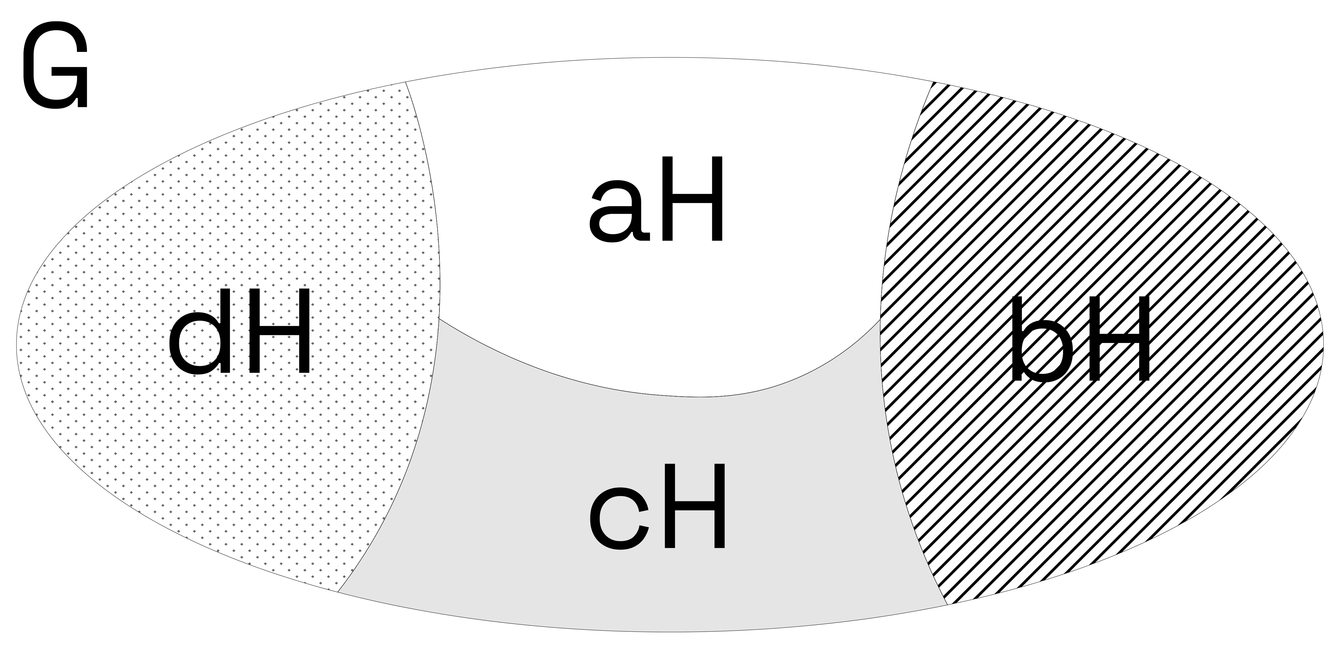
Let $G$ be a group and let $H \subseteq G$ be a subgroup.

Given an element $g \in G$, the left coset of $H$ with respect to $g$ is the set:

$$gH = \{ gh \mid h \in H \}.$$

Similarly, the right coset of $H$ with respect to $g$ is:

$$Hg = \{ hg \mid h \in H \}.$$

In general, left and right cosets are different unless $H$ is a normal subgroup (a concept we will not require here).

Cosets Partition the Group

One of the key properties of cosets is that the set of all left cosets of $H$ in $G$ forms a partition of $G$:

• Every element of $G$ belongs to some left coset.
• Two cosets are either identical or disjoint.

That is, for all $g_1, g_2 \in G$, either $g_1H = g_2H$ or $g_1H \cap g_2H = \emptyset$.

We denote the set of all left cosets of $H$ in $G$ as:

$$G/H = \{ gH \mid g \in G \}.$$

The number of distinct left cosets is called the index of $H$ in $G$, denoted $[G : H]$.

Bijection Between Cosets

All left cosets of a subgroup $H$ have the same size as $H$. In fact, for any $g \in G$, the map:

$$\varphi_g : H \to gH \quad \text{defined by} \quad \varphi_g(h) = gh$$

is a bijection (a one-to-one and onto function).

This means that each coset $gH$ contains exactly $|H|$ elements, and no two cosets overlap. This bijective correspondence is central to the proof of Lagrange’s Theorem, which we will state and prove next.

Lagrange's Theorem

Let $G$ be a finite group and let $H \subseteq G$ be a subgroup. Then:

$$|H| \mid |G| \quad \text{and} \quad |G| = [G : H] \cdot |H|,$$

where $[G : H]$ denotes the number of (left) cosets of $H$ in $G$.

Proof

Since $H$ is a subgroup of $G$, we can form the set of left cosets of $H$ in $G$:

$$G/H = \{gH \mid g \in G\}.$$

We now observe the following facts:

• Disjoint Union: The cosets of $H$ form a partition of $G$. That is, every element of $G$ belongs to exactly one coset. So we can write:

  $$G = \bigsqcup_{i=1}^{[G:H]} g_i H$$

  for some representatives $g_1, \dots, g_{[G:H]} \in G$.

• Equal Size of Cosets: Each left coset $gH$ has the same number of elements as $H$. This follows from the fact that the map $\varphi_g : H \to gH$ given by $h \mapsto gh$ is a bijection.

• Cardinality Calculation: Since there are $[G : H]$ disjoint cosets, each of size $|H|$, and their union gives all of $G$, it follows that:

  $$|G| = [G : H] \cdot |H|.$$

Corollary: Order of an Element

Let $G$ be a finite group with order $n = |G|$, and let $g \in G$. Consider the cyclic subgroup generated by $g$, denoted $\langle g \rangle$.

Let $m = |\langle g \rangle|$, which is by definition the order of the element $g$.

Since $\langle g \rangle$ is a subgroup of $G$, Lagrange's Theorem tells us that the order of any subgroup divides the order of the group. Therefore:

$$m \mid n.$$

In other words the order of any element divides the order of the group.

Elliptic Curves over Finite Fields

Elliptic curves are central objects in modern cryptography. For our purposes, we are interested in elliptic curves defined over finite fields, especially in how they form abelian groups whose structure is relevant to cryptographic protocols — and to attacks.

Fields and Finite Fields

Before we define elliptic curves, we need to understand the algebraic structure they’re defined over: fields.

A field is a set $F$ equipped with two operations:

• Addition $(+)$ and
• Multiplication $(\cdot)$

that satisfy the following properties:

1. Additive group: $(F, +)$ is an abelian group with identity element $0$.
2. Multiplicative group: $(F \setminus \{0\}, \cdot)$ is an abelian group with identity element $1$.
3. Distributivity: For all $a, b, c \in F$, we have $$a \cdot (b + c) = a \cdot b + a \cdot c.$$

Well-known examples of infinite fields include the rational numbers $\mathbb{Q}$, real numbers $\mathbb{R}$, and complex numbers $\mathbb{C}$.

Finite Fields

A finite field (or Galois field) is a field with finitely many elements. The most common finite fields are:

• $\mathbb{F}_p = \mathbb{Z}/p\mathbb{Z}$, the integers modulo a prime $p$
• More generally, $\mathbb{F}_{p^k}$, a degree-$k$ extension field over $\mathbb{F}_p$

In cryptography, we usually work with $\mathbb{F}_p$ where $p$ is a large prime. Arithmetic in such a field is done modulo $p$:

• Addition: $(a + b) \mod p$
• Multiplication: $(a \cdot b) \mod p$
• Inverses exist for all nonzero elements modulo $p$

Finite fields are crucial in elliptic curve cryptography and SNARKs, because they give us a structured but bounded space to compute in — ideal for circuits and modular arithmetic.

The Curve Equation

Let $\mathbb{F}_q$ be a finite field with $q$ elements (typically $q = p$ for some prime $p$, or $q = p^k$ for small $k$). An elliptic curve over $\mathbb{F}_q$ is the set of solutions $(x, y) \in \mathbb{F}_q^2$ to the equation:

$$E: \quad y^2 = x^3 + ax + b,$$

where $a, b \in \mathbb{F}_q$, and the curve is non-singular, meaning:

$$4a^3 + 27b^2 \ne 0.$$

This condition ensures the curve is smooth and has no cusps or self-intersections.

We also include a special point called the point at infinity, denoted $\mathcal{O}$, which acts as the identity element in the group.

Group Law

The points on an elliptic curve $E(\mathbb{F}_q)$, along with $\mathcal{O}$, form an abelian group under a geometric addition law:

• Given two points $P$ and $Q$ on the curve, their sum $P + Q$ is defined via geometric constructions (draw the line through $P$ and $Q$, find its third intersection with the curve, and reflect over the $x$-axis).
• The identity element is $\mathcal{O}$.
• Every point has an inverse (its reflection across the $x$-axis).
• The operation is associative and commutative.

The details of the addition formulas are not important here — only the fact that the group law is well-defined, efficiently computable, and gives the set of curve points the structure of a group.

Base Field vs Scalar Field

When an elliptic curve is defined over a finite field $\mathbb{F}_q$, the set of its points $E(\mathbb{F}_q)$ forms a finite cyclic abelian group.

This means there exists a point $G \in E(\mathbb{F}_q)$ such that repeatedly adding $G$ to itself generates all of the points on the curve. That is:

$$E(\mathbb{F}_q) = \langle G \rangle = \{ \mathcal{O}, G, 2G, 3G, \dots, (r-1)G \},$$

for some prime $r$, where $rG = \mathcal{O}$ and $r$ is the order of the elliptic curve group.

This operation — writing any point as a multiple $[k]G$ of a generator $G$ — is known as scalar multiplication, and the scalars $k$ live in a finite field of size $r$.

This brings us to the distinction between two fields in elliptic curve cryptography:

• The base field $\mathbb{F}_q$: This is the field over which the elliptic curve is defined: $(x,y) \in \mathbb{F}_q \times \mathbb{F}_q$.
• The scalar field $\mathbb{F}_r$: This is the field of integers modulo $r$, used for scalar multiplication $[k]G$, where $k \in \mathbb{F}_r$.

So while the points of the curve live in $\mathbb{F}_q$, the algebra of multiplying a point $G$ by scalars is governed by arithmetic in $\mathbb{F}_r$.

This distinction becomes crucial when reasoning about subgroup structure, constrained scalar ranges, and attack surfaces in cryptographic protocols.

Elliptic Curves in Zero-Knowledge Proof Systems

Elliptic curves are not only used in traditional public-key cryptography, but also play a crucial role in zero-knowledge proof systems, particularly in pairing-based SNARKs like Groth16 and PLONK.

Pairing-Based SNARKs

Proof systems such as Groth16 and PLONK leverage bilinear pairings between elliptic curve groups to achieve:

• Small proof sizes (as small as ~200 bytes),
• Constant-time verification,
• and efficient aggregation.

A pairing is a special function of the form:

$$e : G_1 \times G_2 \to G_T$$

where $G_1$, $G_2$, and $G_T$ are groups associated with an elliptic curve (or pair of curves). The function $e$ satisfies:

• Bilinearity: $e(aP, bQ) = e(P, Q)^{ab}$ for all $P \in G_1$, $Q \in G_2$ and $a, b \in \mathbb{Z}$,
• Non-degeneracy: $e(P, Q) \ne 1$ for some $P$, $Q$,
• and Efficiency: $e$ can be computed efficiently.

Example: Groth16 Pairing-Based Verification Equation

In the Groth16 zk-SNARK protocol, the prover is given:

• A common reference string (CRS) derived from a trusted setup,
• A vector of public inputs $(x_1, \dots, x_\ell)$,
• A vector of private inputs $(x_{\ell+1}, \dots, x_m)$.

Using this data, the prover computes a proof consisting of three group elements:

• $A \in G_1$
• $B \in G_2$
• $C \in G_1$

These group elements encode a commitment to the full assignment $(x_1, \dots, x_m)$ and prove that it satisfies the circuit's constraints without revealing the private inputs.

The verifier is given:

• Verification key elements $[\alpha]_1 \in G_1$, $[\beta]_2 \in G_2$, $[\gamma]_2 \in G_2$, and $[\delta]_2 \in G_2$,
• A set of commitments $\{[K_i]_1\}$ for each public input $x_i$.

Let the public input linear combination be:

$$K_{\text{pub}} = \sum_i x_i [K_i]_1$$

The verifier accepts the proof if the following pairing equation holds:

$$e(A, B) = e(C, [\delta]_2) \cdot e(K_{\text{pub}}, [\gamma]_2) \cdot e([\alpha]_1, [\beta]_2)$$

Here, $e : G_1 \times G_2 \to G_T$ is a bilinear pairing function. This equation ensures the consistency of the proof with the QAP (Quadratic Arithmetic Program) representation of the circuit and the correctness of the witness with respect to the public inputs.

Where Scalars Come In

All the signal involved in the circuit — inputs, outputs, and intermediate signal — are scalars in the finite field $\mathbb{F}_r$, the scalar field of the elliptic curve.

When you write:

signal input a;
signal input b;
signal output c;
c <== a * b;

you're defining a constraint over three scalars in $\mathbb{F}_r$, and these scalars become part of the proof's internal structure. The QAP ensures these values satisfy the circuit's logic, and the pairing check ensures the prover knows such values without revealing them.

BN254 and Missing Range Check Exploit

One of the most widely used elliptic curves in zero-knowledge proof systems is BN254, also known as alt_bn128 in Ethereum. It plays a central role in pairing-based SNARKs like Groth16 and PLONK, and is natively supported in the Ethereum Virtual Machine through precompiles for fast verification.

Curve Overview

BN254 is a Barreto–Naehrig (BN) curve defined over a 254-bit prime field:

• Base field: $\mathbb{F}_p$, where $$p = 21888242871839275222246405745257275088696311157297823662689037894645226208583.$$
• Scalar field: $\mathbb{F}_r$, where $$r = 21888242871839275222246405745257275088548364400416034343698204186575808495617.$$

The curve equation is written in short Weierstrass form:

$$E: y^2 = x^3 + 3 \mod p.$$

BN254 supports efficient bilinear pairings and has been widely adopted in zk-SNARK implementations. However, this curve is not without caveats, especially in the context of constrained environments like smart contracts.

A Real Vulnerability: Missing Nullifier Range Check in ZkDrops

A concrete example of a security issue that stems from mishandling elliptic curve field sizes occurred in a16z’s ZkDrops, a SNARK-based airdrop system. This vulnerability is documented in the 0xPARC zk-bug-tracker.

Summary

ZkDrops requires users to submit a nullifier when claiming an airdrop. This nullifier is supposed to be a unique, deterministic value for each claim and is stored on-chain as a 256-bit integer. The SNARK circuit uses a scalar field of 254 bits (matching the BN254 curve), so any value larger than this is automatically reduced modulo $r$ during proof generation.

However, the smart contract did not verify that the nullifier was within the scalar field range. This allowed users to submit two different nullifiers:

$$x \text{ and } x + r,$$

which both evaluate to the same value modulo $r$ within the SNARK circuit, but appear distinct to the on-chain verifier, which treats them as separate 256-bit integers.

Exploitation

A malicious user could:

1. Claim an airdrop using $x$, which passes circuit verification and is accepted on-chain.
2. Claim the same airdrop using $x + r$, which is the same in the circuit, but different on-chain — thus bypassing the nullifier check.

This effectively allowed the same airdrop claim to be accepted twice.

function collectAirdrop(bytes calldata proof, bytes32 nullifierHash) public {
	require(!nullifierSpent[nullifierHash], "Airdrop already redeemed");

	uint[] memory pubSignals = new uint[](3);
	pubSignals[0] = uint256(root);
	pubSignals[1] = uint256(nullifierHash);
	pubSignals[2] = uint256(uint160(msg.sender));
	require(verifier.verifyProof(proof, pubSignals), "Proof verification failed");
	nullifierSpent[nullifierHash] = true;
	airdropToken.transfer(msg.sender, amountPerRedemption);
}

The Fix

The fix was to add a range check in the smart contract to ensure that the nullifier lies within the scalar field:

require(uint256(nullifierHash) < SNARK_FIELD ,"Nullifier is not within the field");

This guarantees that the on-chain nullifier matches the one used inside the SNARK circuit, preventing duplication via modular reduction.

Baby-Jubjub and Subgroup Range Check Attack

In zk-SNARK circuits based on BN254, all in-circuit arithmetic takes place in the scalar field $\mathbb{F}_r$. To implement elliptic curve operations such as Pedersen hashes or EdDSA signatures within these circuits, we need a curve defined over $\mathbb{F}_r$. This is the role of Baby-Jubjub, a twisted Edwards curve designed for in-circuit use.

Why Baby-Jubjub?

Baby-Jubjub is defined over the BN254 scalar field:

$$r = 21888242871839275222246405745257275088548364400416034343698204186575808495617$$

This allows Baby-Jubjub points to be represented and manipulated using $\mathbb{F}_r$ arithmetic inside a SNARK circuit. The curve has the following structure:

• Form: Twisted Edwards, $$ax^2 + y^2 = 1 + dx^2y^2,$$ with $a = -1$ and a curve-specific constant $d$.
• Total group order: $8 \cdot q$, where $q$ is a large prime and 8 is the cofactor.

This means Baby-Jubjub has a prime-order subgroup of size $q$, but the overall curve has small subgroups due to the cofactor.

The Vulnerability: Missing Scalar Range Check

In a recent audit of AvaCloud, we found a vulnerability in the handling of scalar values used in Baby-Jubjub scalar multiplication. Specifically:

The base point of Baby-Jubjub has order $q < r$ (BN254 scalar field size), but scalar inputs are taken from the full scalar field $\mathbb{F}_r$. Without a check that scalars lie in the correct range (i.e., less than $q$), two distinct scalars can produce the same curve point when multiplied by the base point.

This is because elliptic curve scalar multiplication is defined modulo the group order $q$. As a result:

$$[k]G = [k + n \cdot q]G \quad \text{for any } n \in \mathbb{Z}$$

This means a malicious prover can submit different scalar values — such as $k$ and $k + q$ — that yield the same Baby-Jubjub point. These are aliasing values: different scalars that map to the same point.

Exploitation Scenario

These aliasing values enabled the following attack:

• A user could deposit funds under a Baby-Jubjub public key derived from scalar $k$.
• Later, the same user could generate a second SNARK proof using scalar $k + q$, which still maps to the same Baby-Jubjub point.
• From the circuit’s perspective, both scalars are valid: they result in the same group element.
• From the application’s persptective, the two deposit/withdrawal keys appear distinct, and so the system allowed a second withdrawal under a new-looking but colliding key.

This effectively allowed users to withdraw more funds than they had deposited, by taking advantage of the lack of a scalar range check.

For more details on the Baby-Jubjub scalar aliasing vulnerability, see the full audit report here.

Conclusion

Subgroup attacks arise when a cryptographic system fails to properly constrain the values it operates on — whether those values are scalars, group elements, or curve points. As we've seen, even simple algebraic oversights like a missing range check can have serious consequences.

• In the BN254 nullifier vulnerability, the mismatch between the 254-bit scalar field and 256-bit on-chain integers led to proof reuse and airdrop double-claims.
• In the Baby-Jubjub scalar aliasing issue, failing to constrain scalars to the correct subgroup allowed malicious users to withdraw more than they deposited.

These bugs stem from the same underlying principle: if a value lives in a larger structure than the one intended, and no check is in place to enforce the correct domain, unexpected behavior will follow.

In zero-knowledge cryptography, these issues are especially tricky because of the complexity of proving and verifying computations across different mathematical domains (groups, fields, and curves). Careful validation and awareness of group structure — particularly order, cofactors, and subgroups — is crucial to ensuring soundness.