Understanding Differential Privacy: Part 1

Every useful dataset is also a liability. The same medical records, location traces, and behavioral logs that train better diagnostic models, route ambulances faster, and personalize the products we use are also documents people did not necessarily consent to making public. For most of the last two decades, the industry response to this tension has been a patchwork of fixes: strip the names, blur the timestamps, replace identifiers with hashes, release only aggregates. A line of attacks has made it clear that these fixes do not hold up.

Differential privacy is the field's response to this failure. The guarantee it offers is mathematical, not heuristic. Loosely, an algorithm is differentially private if its output distribution barely changes when any single individual's record is added to or removed from the input. Whatever an attacker learns from the output, they would have learned almost the same thing had you never been in the dataset at all.

In this article we start with the attacks that motivate DP in the first place, then state the formal definition and unpack what its parameters actually mean. From there we look at trust models and deployment settings, the standard mechanisms and their analysis and the accounting machinery that keeps long training runs tractable.

Why privacy fails

Traditional defenses have repeatedly proven inadequate against adversaries with serious computational tools and access to auxiliary datasets. The cleanest way to see why is to look at the attacks that defeat them.

Linkage attacks

A linkage attack works by joining a "de-identified" dataset against an external source that shares some attributes with it. Even when names are stripped, the remaining fields are often unique enough in combination to pin a row to a person. Sweeney's 1997 attack re-identified medical records by joining them against voter registration data, showing that the combination of ZIP code, birth date, and gender was enough to re-link supposedly anonymous records to individuals. The same template defeated the Netflix Prize release: Narayanan and Shmatikov showed that the released ratings data could be linked to IMDb to recover the viewing histories of specific users. Linkage attacks are the proof that "anonymization" is not a property you can verify by inspecting a dataset on its own, it depends on what other data happens to exist in the world.

Reconstruction attacks

Reconstruction attacks, on the other hand, try to recover the rows themselves from a series of aggregate releases. The foundational result is due to Dinur and Nissim, who proved that releasing too many highly accurate statistics about a dataset allows an adversary to reconstruct a large portion of the original records, saying that overly accurate answers to too many queries can destroy privacy. This is not a theoretical worry. Working with the published statistical summaries from the 2010 U.S. Census, researchers at the Census Bureau were able to reconstruct individual-level records. This result directly motivated the Bureau's decision to adopt DP for subsequent releases.

Differencing attacks

Differencing attacks weaponize the gap between two aggregate queries that overlap in everything except one person. If a system reports the average salary of "employees in department X" and "employees in department X excluding Alice," subtracting one from the other gives Alice's salary directly, regardless of how many people are in the average. A version of this attack surfaced on Facebook's advertising platform: by crafting highly specific target audiences and comparing the resulting ad reach statistics, an attacker could infer sensitive traits, including sexual orientation and medical conditions, about individual users.

Membership inference attacks

Membership inference asks a narrower but often equally damaging question: was this specific person's record in the dataset? In medical or genomic settings, the answer alone is sensitive, confirming that someone was in a cohort of HIV patients or rare-disease participants is already a disclosure. Shokri et al. showed that trained models leak membership, allowing an adversary with only query access to the model to tell, with non-trivial accuracy, whether a particular record had been in the training set.

The core promise of differential privacy

Rather than asking whether a dataset is "anonymous," DP asks a question about an algorithm: if you ran it on a dataset that differs by one person, how different would the output look? If the answer is almost the same, with high probability, the algorithm is private.

Neighboring datasets

The basic unit of analysis is a pair of neighboring datasets, that is two datasets that are identical except for the data of a single individual. We write $D \sim D'$ to mean that $D'$ can be obtained from $D$ by adding or removing one record. This is the add-or-remove criterion. Two alternative conventions appear in the literature. The replace-one criterion says that $D'$ is obtained from $D$ by replacing one record with a different record; the zero-out criterion replaces a record with a designated "zero" value rather than removing it. The add-or-remove and zero-out variants give semantically equivalent guarantees with respect to $\varepsilon$, while replace-one is roughly twice as strong, since a replacement is effectively an add plus a remove.

A related choice is what counts as a "record" in the first place. This is the unit of privacy. Example-level (or sample-level) DP treats each row of the dataset as the protected unit, while user-level DP protects all of the data contributed by a single user, even when one user contributes many rows. The difference matters whenever individuals contribute repeatedly like a user with months of typing logs or a patient with many medical records, because example-level guarantees can lessen when one person's records are correlated across many rows.

Formal definition

With neighbors in hand, the standard definition is short. A randomized mechanism $\mathcal{A}$, mapping datasets to some output space $\mathcal{R}$, satisfies pure $\varepsilon$-DP if, for every pair of neighboring datasets $D \sim D'$ and every measurable set of outputs $S \subseteq \mathcal{R}$,

$$\mathbb{P}[\mathcal{A}(D) \in S] \;\leq\; \exp(\varepsilon) \cdot \mathbb{P}[\mathcal{A}(D') \in S].$$

In many practical settings, especially in machine learning, pure $\varepsilon$-DP is too restrictive, the standard relaxation is approximate $(\varepsilon, \delta)$-DP:

$$\mathbb{P}[\mathcal{A}(D) \in S] \;\leq\; \exp(\varepsilon) \cdot \mathbb{P}[\mathcal{A}(D') \in S] + \delta.$$

Setting $\delta = 0$ recovers pure $\varepsilon$-DP. Allowing $\delta > 0$ tolerates a small probability that the multiplicative bound fails to hold.

What $\varepsilon$ and $\delta$ actually mean

The parameter $\varepsilon$ controls how much an adversary's inference about any one record can shift when that record is added or removed. A smaller $\varepsilon$ means stronger privacy, so the output is less sensitive to any individual's data, while a larger $\varepsilon$ means weaker guarantees. At $\varepsilon = 0$ the output is statistically independent of the input, which makes it useless. There is no single "right" value; for common statistical queries $\varepsilon$ is typically chosen below 1, whereas in deep learning settings it is often relaxed to around $\varepsilon = 10$.

The parameter $\delta$ needs extra care because it allows a small probability of a complete privacy failure. Recall that $(\varepsilon,\delta)$-DP requires that for neighboring datasets $D$ and $D'$ and every possible output event $S$,

$$\Pr[M(D)\in S] \leq e^\varepsilon \Pr[M(D')\in S] + \delta.$$

Now consider a deliberately terrible mechanism: it takes a dataset $D$ of $n$ people, chooses one person uniformly at random, and releases that person’s full record with no noise. Fix one individual, say Alice, and let $S$ be the event that the mechanism outputs Alice’s record. If Alice is in the dataset $D$, then

$$\Pr[M(D)\in S] = \frac{1}{n}.$$

But in the neighboring dataset $D'$, where Alice’s record has been removed, the mechanism cannot output her record at all, so

$$\Pr[M(D')\in S] = 0.$$

Plugging this into the DP definition gives

$$\frac{1}{n} \leq e^\varepsilon \cdot 0 + \delta,$$

so $\delta \geq \frac{1}{n}.$

This means that even an obviously unsafe mechanism can satisfy $(\varepsilon,\delta)$-DP if $\delta$ is at least about $1/n$. The reason is that the probability of exposing any fixed individual is hidden inside the allowed failure probability $\delta$.

This is why $\delta$ should be much smaller than $1/n$. If $\delta$ were on the order of $1/n$, then in a dataset with $n$ people, the guarantee could still allow roughly one catastrophic disclosure in expectation. More generally, if each record has failure probability about $\delta$, then the expected number of failures across the dataset is about $\delta n$. So reporting an $(\varepsilon,\delta)$ guarantee without saying what $\delta$ is or choosing $\delta \approx 1/n$ is much weaker than it may sound.

Trust models: who sees the raw data?

The formal definition of DP says nothing about who runs the mechanism. In practice that matters a great deal, because privacy guarantees on a final output do not protect users from whoever holds the raw data before noise is added. Trust models are the standard way to organize this question, they specify, for each part of the pipeline, what an adversary is assumed to see and which failures the protocol is supposed to survive.

Central DP

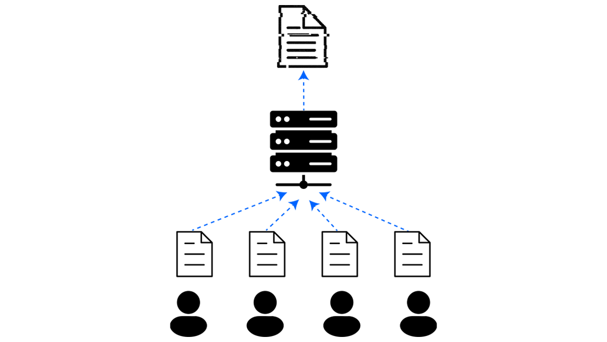
Central DP is the classical setting and the easiest to reason about. A trusted curator (or a trusted aggregator) collects raw, unperturbed data from users, applies a DP mechanism, and releases outputs that satisfy formal DP guarantees. Users must trust this aggregator both to safeguard the raw data and to implement the mechanism correctly. The adversary is assumed to observe only the final output. Because the curator has access to unperturbed data, only a small amount of noise is needed, which is why central DP typically achieves the highest utility of any setting. The standard applications that fit this profile are centralized analytics and ML pipelines, and research analyses under strong governance, including healthcare studies that protect patient information.

The weakness of central DP is exactly what makes it convenient: it concentrates risk on the curator. If the curator is breached, malicious, or compelled to hand over data, DP on the final output is no comfort to people whose raw records have already been exfiltrated. A 2018 Google+ leak affected hundreds of thousands of users, a separate Google+ API bug later that year exposed the data of 52.5 million users, and a 2019 Facebook breach exposed IDs, phone numbers, and names of hundreds of millions. Even reputable, well-resourced curators are at risk.

Local DP

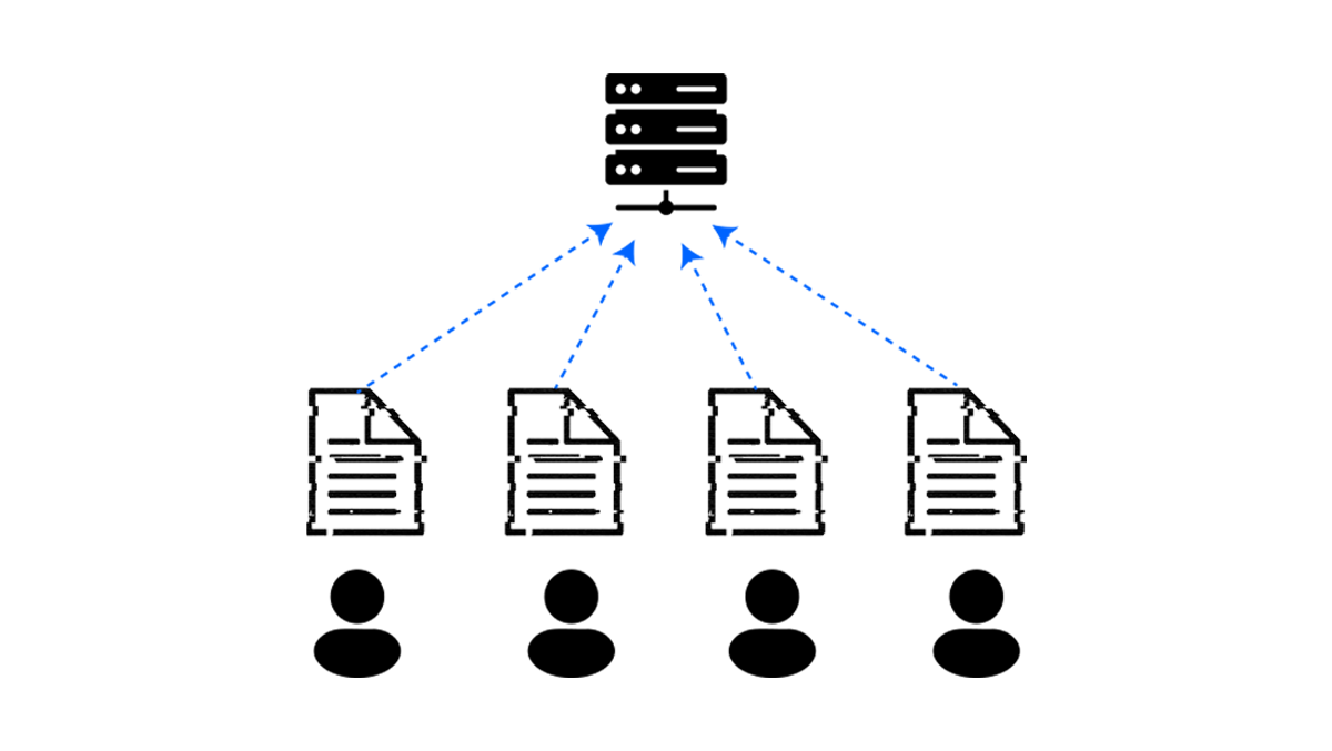
Local DP eliminates the trusted curator by moving the noise onto the user's device. Each user applies a predefined randomized mechanism to perturb their own data before anything is sent to a server. As a result, the server never sees the raw values, and privacy holds regardless of the aggregator's behaviour.

The price is utility. Because every user adds noise independently, local DP typically requires much larger per-user noise than the central setting, which translates to lower accuracy. Local DP is best suited for very large user bases performing simple aggregate analyses like Apple's iOS telemetry for emoji usage and typing behaviour.

Shuffle DP

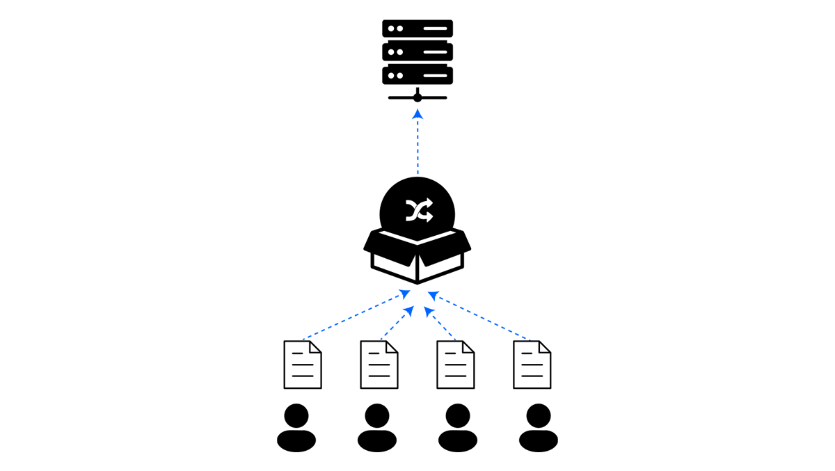
Shuffle DP introduces a semi-trusted shuffler between users and the aggregator: each user sends their data through the shuffler, which removes any user identifiers and randomly permutes the reports before they reach the aggregator. The aggregator then adds a small amount of noise to the shuffled aggregate. Deployments include federated learning with secure aggregation and sparse location heatmaps generated from many users' reports without any central trusted curator.

The catch is the trust assumption on the shuffler. If the shuffler colludes with the aggregator the model effectively collapses, so it is usually implemented with cryptographic protections (secure aggregation, mixnets) ensuring that no single party can both see identifiers and read message contents.

Pan-privacy

Pan-privacy is conceptually distinct from the three settings above, it introduces the notion of time. Users contribute their data to the server sequentially; once collection is complete, the output is released. The trust model is time-sensitive meaning users trust the server at the moment they hand over their data, but not necessarily after. A pan-private algorithm guarantees that if the server is later compromised, the data already in the server stays private. In practice, pan-privacy is rarely deployed standalone. It is best thought of as a property layered on top of a central or distributed system.

Deployment settings

Trust models define who is trusted and who is adversarial. Deployment settings define the circumstances: where the data is created, where it can move, who is allowed to process it, and what infrastructure already exists.

If the data is generated on millions of phones, the system may need client-side or federated methods. If the data already lives in a central statistical agency or hospital system, a trusted-curator model may be realistic. If no single party is allowed to see the full dataset, then distributed protocols become necessary.

Centralized systems

The centralized setting is the one most DP tooling is designed for. A single server (or cluster) holds the dataset, runs the analysis or training pipeline, and produces a private output.

The curator has access to unperturbed data, so noise can be calibrated once at the aggregate level. The implementations are also relatively well-developed, with libraries like TensorFlow Privacy and Opacus.

Local/client-side systems

When data cannot be centralized, the noise has to move to the device. A client-side deployment runs a small randomizer on each user's device, applies it to a single data point (or a small per-user payload), and transmits only the perturbed report. The server's job is reduced to aggregation. Examples of this setting are Google's RAPPOR, used for collecting Chrome browser-configuration data via randomized response, and Apple's iOS telemetry pipeline, which uses local DP for emoji usage, typing behaviour, and Safari domain popularity measurements.

Distributed/federated systems

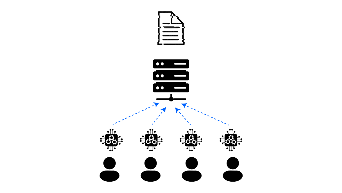
The third architecture is federated: a coordinating server orchestrates training across many participants that keep their data local such as phones, hospitals and banks. Each participant computes updates (typically gradients) on its own data and sends those updates to the server, which aggregates them into a global model. The data itself never moves.

Federated learning becomes a DP system when noise is added to the updates: each device clips and noises its own gradient contribution, the server sums the contributions without seeing individual updates, and the privacy budget is tracked across rounds.

The engineering complexity is significantly higher than in either of the other two settings. Federated systems have to handle heterogeneous data distributions across participants, devices that drop out mid-round, asynchronous availability, and communication-bandwidth constraints. Frameworks like Flower and TensorFlow Federated have made these systems much more tractable to build than they were five years ago, but federated DP remains the most operationally demanding of the three architectures. You can read more about Federated Learning in our previous post.

Where noise enters the pipeline

The trust model fixes who is allowed to see what, and the deployment setting fixes what the system physically looks like. Inside that frame, there is one more decision with large consequences for utility and accounting: at which point in the pipeline does the noise actually enter?

Input perturbation

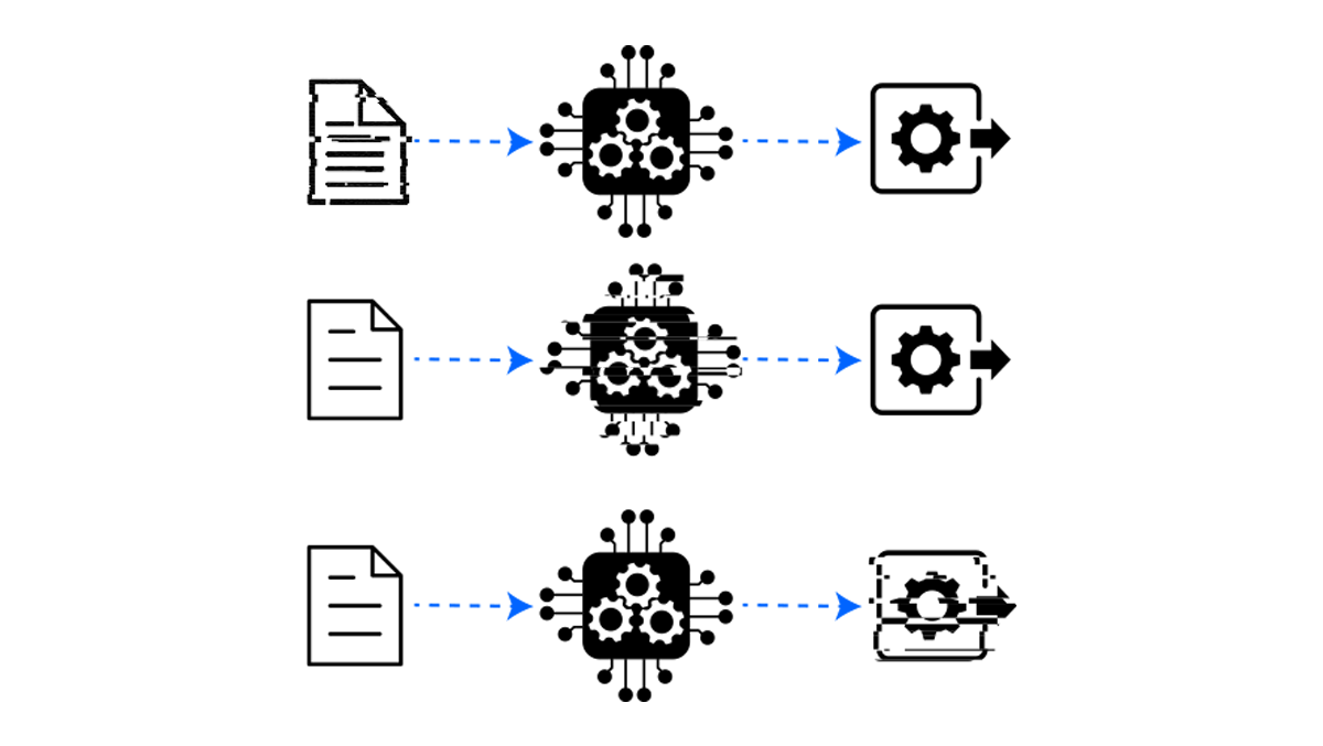
Input perturbation adds noise to the data itself, before any training. After that, every downstream computation inherits the guarantee for free. This is what powers DP synthetic data releases and what makes local DP work: each user randomizes their record, and anything the server does with it is private by default.

The win is reusability. One private dataset can train many models, support hyperparameter sweeps, and feed comparisons without spending any more budget. It also gives the strongest guarantees of the three options.

The cost is utility. Noise has to be calibrated for the worst-case downstream use, not the actual one, which usually means more noise than any single task would need. Local-DP training and DP synthetic data both pay heavily for this, which is why input-level DP is often the hardest to deploy well.

Training-time perturbation

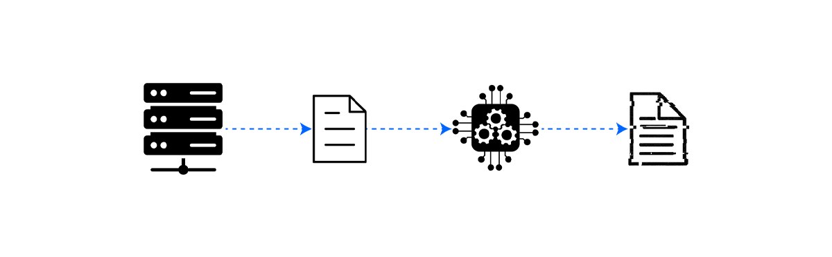
Training-time perturbation modifies the algorithm rather than the data. The curator holds the dataset privately, the training procedure injects noise during optimization, and the released model is the differentially private object. Every prediction the model later produces is also private.

The advantage over input perturbation is utility. Because the optimizer sees clean data during training, noise can be calibrated against what the optimization actually needs to tolerate, not against a worst-case downstream query. The advantage over output perturbation is scope: the model itself is private, so once it is trained it can be released, served, or shared.

The costs arise from hyperparameter sensitivity, the computational overhead of per-example gradient computation, and the need for careful accounting across long training runs.

Output perturbation

Output perturbation leaves the data and the algorithm alone and adds noise at the end of the pipeline, when the answer is returned. The canonical example is a privacy-preserving prediction API: the model itself isn't released, and each query is perturbed enough that no single prediction reveals much about any one training example.

This works best when the number of queries is tightly bounded. For a system that releases a handful of aggregate statistics from a frozen dataset, perturbing the outputs directly is simple and easy to account for.

The catch is that the budget scales with queries. Every output draws from the same finite $\varepsilon$, so a system answering many queries eventually runs out. For ML specifically, training-time DP usually gives a better privacy-accuracy trade-off, especially with large inference budgets or large training sets and it protects the model parameters too, which output perturbation doesn't.

Mechanisms, sensitivity, and DP variants

Every DP system needs a concrete mechanism: figure out how much one person's contribution can shift the output (sensitivity), pick a noise distribution whose spread covers that shift, and verify that the resulting algorithm fits one of the DP definitions.

Sensitivity

Sensitivity is the bridge between a function and the amount of noise required to make it private. It measures the worst-case change a single person's data can produce in the function's output. Formally, for a query function $f: \mathcal{D} \to \mathbb{R}^d$ and the set $\mathcal{N}$ of all neighboring dataset pairs, the global $\ell_p$-sensitivity of $f$ is

$$\Delta_f^p \;=\; \max_{(D, D') \in \mathcal{N}}\;\|f(D) - f(D')\|_p,$$

where $\|\cdot\|_p$ is the $\ell_p$-norm. Two specializations matter most: $\ell_1$-sensitivity (used by the Laplace mechanism) and $\ell_2$-sensitivity (used by the Gaussian mechanism).

The amount of noise a DP mechanism must add is directly proportional to $\Delta^p_f$. Queries with higher sensitivity require more noise to mask the influence of any one individual. Here are some examples for better intuition:

• A counting query that returns the number of records satisfying a predicate has $\Delta^1_f = 1$, since adding or removing one record changes the count by at most one.
• A sum-of-ages query has $\Delta^1_f$ equal to the maximum possible age, since one added record can shift the total by that amount.

In practice, sensitivity is often unbounded or hard to estimate. The standard fix is clipping: bound the per-record contribution (or in ML, the per-example gradient) to a fixed norm $C$, which forces $\Delta^p_f \leq C$ by construction. Clipping introduces a bias–variance trade-off: too tight a clip distorts the function being computed, too loose a clip requires too much noise.

Laplace mechanism

The Laplace mechanism is the simplest DP building block. It adds noise drawn from the Laplace distribution. The Laplace distribution centered at zero with scale parameter $b > 0$ has density

$$g(u) \;=\; \frac{1}{2b}\exp\!\left(-\frac{|u|}{b}\right),$$

variance $2b^2$, and exponential tails. We write $\mathrm{Lap}(b)$ for this distribution.

For a query $f: \mathcal{D} \to \mathbb{R}^d$, the Laplace mechanism adds independent noise to each coordinate:

$$\mathcal{A}_L(D; f, \varepsilon) \;=\; f(D) + (Y_1, Y_2, \ldots, Y_d), \quad Y_i \overset{\mathrm{iid}}{\sim} \mathrm{Lap}\!\big(\Delta^1_f / \varepsilon\big),$$

and the resulting mechanism satisfies pure $\varepsilon$-DP.

A worked example: suppose a security analyst wants to release the count of log entries matching a particular malware signature. Adding or removing one entry changes the count by at most one, so $\Delta^1_f = 1$, and the mechanism returns

$$\mathcal{A}_L(D; f, \varepsilon) \;=\; f(D) + Y, \quad Y \sim \mathrm{Lap}(1/\varepsilon).$$

At $\varepsilon = 1$, the noise has standard deviation $\sqrt{2} \approx 1.41$, so the published count is usually within a handful of the true value yet no adversary can determine from the output whether any specific log entry was included. The Laplace mechanism is the default tool for releasing counts, sums, and averages under pure $\varepsilon$-DP.

Gaussian mechanism

The Gaussian mechanism is the workhorse for $(\varepsilon, \delta)$-DP. The structure mirrors Laplace, but the noise is Gaussian and the calibration is to $\ell_2$-sensitivity rather than $\ell_1$.

For $f: \mathcal{D} \to \mathbb{R}^d$, the Gaussian mechanism is

$$\mathcal{A}_G(D; f, \varepsilon, \delta) \;=\; f(D) + (Y_1, \ldots, Y_d), \quad Y_i \sim \mathcal{N}(0, \sigma^2),$$

with

$$\sigma \;=\; \frac{\Delta^2_f \sqrt{2 \ln(1.25/\delta)}}{\varepsilon}.$$

This noise scale guarantees that the mechanism satisfies $(\varepsilon, \delta)$-DP.

Why prefer Gaussian over Laplace? In low dimensions, often you don't. In high dimensions, Gaussian has practical advantages. $\ell_2$-sensitivity is typically much smaller than $\ell_1$-sensitivity: for a $d$-dimensional vector each of whose entries can change by at most one, $\ell_1$ grows as $d$ while $\ell_2$ grows only as $\sqrt{d}$ which means less total noise is required.

A concrete example: a hospital publishes the average BMI of 100 individuals, with BMI bounded in the physiological range $[10, 60]$. The maximum any one person can shift the average is $(60 - 10)/100 = 0.5$, so $\Delta^2_f = 0.5$. To achieve $(\varepsilon, \delta) = (1, 10^{-5})$,

$$\sigma \;=\; \frac{0.5 \cdot \sqrt{2 \ln(1.25/10^{-5})}}{1}.$$

About 99.7% of Gaussian draws fall within $\pm 3\sigma (≈3⋅2.42=7.26)$, so the published average lies within roughly that range of the truth. It's wide enough to hide any single contribution, narrow enough to remain useful in practice.

Randomized response

Laplace and Gaussian assume a trusted curator who already has the data. Randomized response is the canonical mechanism for local DP. The user randomizes their own answer before sending anything to anyone.

The classical version handles a sensitive yes/no question. Each respondent flips a fair coin, answers truthfully if it lands heads, and otherwise flips a second coin to choose "yes" or "no" at random. The probabilities work out as:

• If the true answer is yes, the respondent reports yes with probability $\tfrac{1}{2} + \tfrac{1}{2} \cdot \tfrac{1}{2} = 0.75$.
• If the true answer is no, the respondent reports yes with probability $\tfrac{1}{2} \cdot \tfrac{1}{2} = 0.25$.

The privacy loss on observing a "yes" is therefore $\ln(0.75/0.25) = \ln 3$, and on observing a "no" it is $-\ln 3$. The maximum across all outputs defines $\varepsilon$, so the classical randomized response mechanism satisfies $\varepsilon$-local DP with $\varepsilon = \ln 3 \approx 1.1$. The analyst can still estimate the population proportion accurately: knowing the randomization rule, they can subtract off the share of responses that are random and recover an unbiased estimate of the true rate.

Personalized DP

Standard DP applies the same budget to every individual. Personalized DP (PDP) loosens this by assigning each user $i$ their own $\varepsilon_i$, so users with stronger privacy preferences or with more sensitive data get tighter guarantees. This requires modifying the underlying mechanism to enforce the per-user budgets.

Two related notions sit nearby and are sometimes used interchangeably with PDP, but should be distinguished. Heterogeneous DP assigns different privacy levels by system-level factors like data sensitivity, model roles, or organizational policies, rather than by explicit user preference; it has been applied in federated learning settings where participants come with different governance requirements. Sensitive privacy adapts $\varepsilon$ to each record's "outlierness," providing weaker protection for rare records and stronger protection for typical ones. This is useful in tasks like anomaly detection, where strict uniform DP is effectively incompatible with the task.

Privacy accounting

Training a model takes thousands of rounds, and each round is another release on the same data. The training algorithm itself comes in Part 2, but the accounting machinery is worth setting up now.

This section is about tracking how privacy loss adds up across rounds. The naive answer is to sum the per-round $\varepsilon$'s. This works but gets useless fast once the number of rounds is large. Tighter accounting is what keeps the final guarantee meaningful.

Composition

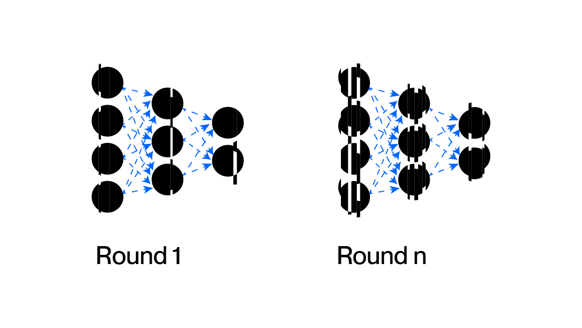
The starting point is sequential composition. If you release the outputs of $k$ mechanisms $\mathcal{A}_1, \ldots, \mathcal{A}_k$ that each satisfy $(\varepsilon_i, \delta_i)$-DP, the combined release satisfies $\left(\sum_{i=1}^k \varepsilon_i,\; \sum_{i=1}^k \delta_i\right)$-DP. This is what 'privacy budget' actually means: every release spends some, and the totals accumulate by addition.

Consider a thought experiment: a training run of $T = 10{,}000$ gradient steps, each with a per-step $\varepsilon$ of $0.01$ which would already be a tight per-step bound. Naive composition reports a final $\varepsilon = T \cdot 0.01 = 100$, a guarantee so loose it conveys essentially nothing about the actual privacy of the trained model. The mechanism leaks much less than this; the bound is just bad.

The intuition for why sequential composition is loose: it adds up the worst case over every step, treating every step's privacy loss as if it were maximal and all pulling in the same direction. Tighter accounting comes from refusing to take the worst case quite so literally.

Advanced composition

The first real refinement is advanced composition. For $k$ mechanisms each satisfying $(\varepsilon, \delta)$-DP, the composition satisfies $(\varepsilon', k\delta + \delta')$-DP for any $\delta' > 0$, where

$$\varepsilon' \;=\; \sqrt{2k \ln(1/\delta')}\,\varepsilon \;+\; k\varepsilon(e^{\varepsilon} - 1).$$

For small $\varepsilon$, the second term is negligible and the bound simplifies to

$$\varepsilon' \;\approx\; \sqrt{2k \ln(1/\delta')}\,\varepsilon \;+\; k\varepsilon^2.$$

The key change is the $\sqrt{k}$ scaling: the dominant term grows as the square root of the number of compositions, not linearly. The price is a small extra $\delta'$. Intuitively, per-step privacy losses behave like noisy random variables that partially cancel rather than always conspiring; their sum has $\sqrt{k}$-style fluctuations, not $k$-style.

Replaying our thought experiment with advanced composition and $\delta' = 10^{-5}$:

$$\varepsilon' \;\approx\; \sqrt{2 \cdot 10{,}000 \cdot \ln(10^5)} \cdot 0.01 \;+\; 10{,}000 \cdot (0.01)^2 \;\approx\; 4.8 + 1.0 \;=\; 5.8.$$

The same algorithm now reports an $\varepsilon$ around 6 instead of 100, which is better, but still too loose for many real training runs. For long training runs in particular, advanced composition remains overly conservative, which is exactly the gap that the moments accountant was designed to close.

The moments accountant

The big jump came with the moments accountant. The idea is to stop bounding the worst-case privacy loss and start tracking its statistical behaviour directly.

For each step, define the privacy loss random variable

$$c(o;\, \mathcal{M}, D, D') \;=\; \log \frac{\mathbb{P}[\mathcal{M}(D) = o]}{\mathbb{P}[\mathcal{M}(D') = o]},$$

where $o$ is drawn from $\mathcal{M}(D)$. Sequential composition bounds the supremum of this random variable. The moments accountant instead tracks its log moments:

$$\alpha_\mathcal{M}(\lambda) \;=\; \log \mathbb{E}_{o \sim \mathcal{M}(D)}\!\left[\exp\!\big(\lambda \cdot c(o;\, \mathcal{M}, D, D')\big)\right].$$

For the subsampled Gaussian mechanism with sampling rate $q = B/n$ (batch size over dataset size) and noise multiplier $\sigma$, the derived bound is

$$\alpha(\lambda) \;\leq\; \frac{q^2 \lambda(\lambda+1)}{(1-q)\sigma^2} \;+\; O\!\left(\frac{q^3}{\sigma^3}\right).$$

Three things make this powerful. First, log moments add cleanly under composition: after $T$ steps, the cumulative log moment is bounded by $T \cdot \alpha(\lambda)$. Second, the bound scales as $q^2$ in the sampling rate, which captures the privacy amplification from subsampling (the next subsection). Third, the cumulative log moment converts back into a final $(\varepsilon, \delta)$ via a tail bound,

$$\delta \;=\; \min_\lambda \exp\!\big(\alpha_\mathcal{M}(\lambda) - \lambda \varepsilon\big),$$

which is then optimized over the moment order $\lambda$ to give the tightest possible $(\varepsilon, \delta)$ pair.

The improvement over advanced composition is order-of-magnitude in real scenarios. Consider training with sampling rate $q = 0.01$, noise multiplier $\sigma = 4$, and $\delta = 10^{-5}$. Each epoch runs $T = E/q = 100E$ steps. At $E = 100$ epochs (10,000 steps), advanced composition reports $\varepsilon = 9.34$ while the moments accountant reports $\varepsilon = 1.26$. At $E = 400$ epochs (40,000 steps), advanced composition gives $\varepsilon = 24.22$ and the moments accountant gives $\varepsilon = 2.55$. Same algorithm, same noise, much tighter story about what it leaks.

Privacy amplification by subsampling

A separate phenomenon, tied to everything above, is privacy amplification by subsampling. The intuition is short. Suppose a base mechanism $\mathcal{M}$ satisfies $\varepsilon$-DP when applied to a fixed dataset. Now consider the subsampled mechanism $\mathcal{M}_q$ that first draws each record independently with probability $q$ (Poisson subsampling), then applies $\mathcal{M}$ to the subsample. Any particular record appears in the subsample only with probability $q$, so an adversary observing $\mathcal{M}_q$'s output can't tell whether the record was excluded by the subsampler or simply absent from the dataset. The amplified guarantee is approximately

$$\big(\log(1 + q(e^{\varepsilon} - 1)),\; q\delta\big)\text{-DP},$$

which for small $\varepsilon$ is close to $(q\varepsilon, q\delta)$-DP. A per-step $\varepsilon$ of $0.5$ at full batch becomes a per-step $\varepsilon$ of around $0.005$ when the sampling rate is $q = 0.01$, that's roughly a hundredfold tightening.

Conclusion

Differential privacy didn't replace ad-hoc anonymization because it looked nicer on paper. It replaced it because every other approach failed. The four attacks at the start of this article aren't exotic edge cases. They're what happens when you release data without a formal model of what an adversary can do with it. DP starts from the opposite assumption: the adversary is allowed to be clever, well-resourced, and to have arbitrary side information but the guarantee has to hold anyway. Much of the framing and many of the examples in this article draw on "A Comprehensive Guide to Differential Privacy: From Theory to User Expectations", which we recommend if you want a deeper survey of the field.

Coming in Part 2

Part 2 picks up where the accounting section leaves off. We'll work through DP-SGD, the training algorithm that turns all of this machinery into a private model, and then put it to use. The plan is to train a simple model on the same dataset twice, once normally and once with DP-SGD using one of the libraries mentioned above, and look at what the privacy-utility trade-off actually costs in practice. How big is the accuracy gap at different values of $\varepsilon$. How clipping and noise interact during real training. What the reported $(\varepsilon, \delta)$ at the end actually tells you about the model.