Understanding Differential Privacy: Part 2

Part 1 covered how DP composes across rounds, how the moments accountant tightens what naive composition gets wrong, and how Poisson subsampling magnifies the per-step guarantee. What we didn’t do is put any of it to work.

In this post, we’ll walk through DP-SGD, the algorithm that turns all of this into a private model. We’ll look at how it shows up in real deployments, including Google’s VaultGemma. Then we’ll train a small model on CIFAR-10 twice, once normally and once with DP, and look at what the privacy-utility trade-off actually costs.

DP-SGD for private model training

Training a neural network involves hundreds of thousands of gradient updates, and you have to track the privacy budget across all of them, or the final guarantee means nothing. Differentially Private SGD is the standard tool for this. It started out with simple models, got adapted to deep learning, and became practical once the moments-accountant technique came along. Every modern DP library implements it: TensorFlow Privacy, Diffprivlib, PyTorch Opacus.

The construction modifies standard SGD in three places. Per-example gradients replace the batch-averaged gradient. Each one gets clipped to bound its influence. Gaussian noise is added before the optimizer step. Each of these is worth walking through on its own.

Per-example gradients

Standard SGD computes one gradient per mini-batch by averaging the per-example losses and backpropagating once. This is fast because modern accelerators are designed for exactly this kind of batched computation, but it produces a single gradient vector with no record of how each individual example contributed. DP-SGD needs that record. To bound the influence any one training example can have on the model update, the mechanism has to be able to bound and noise each example’s contribution individually, which means computing the gradient $g_i = \nabla_\theta \mathcal{L}(\theta, x_i, y_i)$ separately for every example in the batch, before any averaging.

In practice, per-example gradient computation is the main source of DP-SGD’s computational overhead. It limits hardware acceleration, increases memory consumption, and often forces smaller batch sizes or specialized implementations. Production frameworks recover some of the lost parallelism through vectorized per-example gradient implementations (Opacus’ GradSampleModule, JAX’s vmap, hooks in TensorFlow Privacy), but per-example gradients still cost more time and memory than a standard backward pass.

Gradient clipping

With per-example gradients in hand, the next step is to bound their $\ell_2$-norm. DP-SGD clips each individual gradient to a maximum norm $C$:

$$g_i \leftarrow\frac{g_i}{\max\left(1,|g_i|_2 / C\right)}.$$

Gradients smaller than $C$ in norm pass through unchanged; gradients larger than $C$ are rescaled to exactly norm $C$. This guarantees that no single example’s gradient has too much influence on the update.

The choice of $C$ matters. If you set $C$ too small, many gradients are excessively clipped, which biases the optimizer and degrades accuracy. If you set $C$ too large, individual examples exert more influence on the update, which requires larger noise to retain the same privacy guarantee.

Gaussian noise

Clipping gives a bounded-sensitivity gradient estimate. Adding Gaussian noise turns it into a private one. The DP-SGD update is

$$\tilde g \leftarrow \frac{1}{B} \sum_{i=1}^{B} g_i + \mathcal{N}\left(0, \sigma^2 C^2 \mathbf{I}\right),$$

where $B$ is the batch size, $C$ is the clipping norm, $\sigma$ is the noise multiplier, and $\mathbf{I}$ is the identity matrix. The Gaussian noise has the same scale in every direction of the model’s parameter space. The noisy gradient $\tilde g$ then feeds the standard SGD update,

$$\theta \leftarrow \theta - \eta \tilde g,$$

where $\eta$ is the learning rate.

DP-SGD also leans heavily on the privacy amplification by subsampling we covered in Part 1. Mini-batches are commonly constructed by Poisson subsampling, where each record is included in each batch independently with a fixed probability $q$. Because any particular record participates in any particular batch only with probability $q$, a single step leaks much less about that record than a step on a fixed-membership batch would.

Hyperparameter tuning under DP

DP-SGD has more hyperparameters than standard SGD. $C$ and $\sigma$ get added on top of the usual learning rate, batch size, and number of epochs. Tuning them all from scratch on private data is expensive, both in compute and in privacy budget.

The recommended strategy is:

1. Start from non-private training to fix sensible defaults for learning rate, batch size, and epoch count.
2. Sweep the clipping norm $C$ with $\sigma = 0$ to find the smallest value that preserves utility.
3. Compute the $\sigma$ that satisfies the target $(\varepsilon, \delta)$ via a privacy accountant.
4. Tune the learning rate with $C$ and $\sigma$ fixed.

This sequence isolates each parameter’s contribution and keeps the number of private runs small.

DP in the wild

The theory above has been in production for a while. DP moved from research to deployment in stages: the US Census Bureau’s 2020 release was the first national statistical release under formal DP; Google’s RAPPOR has collected Chrome browser-configuration data under local DP since 2014; Apple’s iOS pipeline applies local DP to emoji usage, typing behavior, and Safari domain popularity. All of those were on classical statistical workloads, where DP’s noise costs were manageable, and the analyses themselves were simple.

Extending the same machinery to large language models took another decade of accounting improvements, scaling laws research, and infrastructure. The release of VaultGemma in late 2025 is the cleanest current example of what that looks like in practice.

VaultGemma

VaultGemma is a 1-billion-parameter language model released in September 2025 by Google Research and DeepMind. It is built on the Gemma 2 decoder-only transformer architecture with sequence length deliberately limited to 1,024 tokens to make private training computationally feasible. The keyword is from scratch: VaultGemma is the largest open model fully pre-trained under differential privacy, rather than DP fine-tuned on top of a non-private base.

VaultGemma’s guarantee is $(\varepsilon \leq 2.0 , \delta \leq 1.1 \times 10^{-10})$, defined at the 1,024-token sequence level. The training algorithm is DP-SGD with gradient clipping at $C = 1.0$ and Gaussian noise at $\sigma = 0.614$. Batches use truncated Poisson subsampling, which keeps batch sizes fixed and preserves the privacy amplification of ordinary Poisson sampling without the throughput hit from variable batches. Training ran for 100,000 iterations at an expected batch of about 518,000 tokens, on 2,048 TPUv6e chips. The pipeline is built on JAX Privacy, with vectorized per-example clipping and gradient accumulation.

The companion paper on scaling laws for DP language models is, in some ways, the bigger contribution. Its main finding is that the noise-batch ratio is the dominant performance lever under DP. Larger batches, more iterations, or more training data each shrink this ratio and partially pay down the cost of the noise. The optimal recipe flips from the non-private case: smaller models on much larger batches outperform bigger models on tighter batches. Batch size is what makes the per-step noise tolerable, so that’s where the compute goes. VaultGemma’s actual training loss landed within 1% of what the scaling law predicted.

On benchmarks, VaultGemma trails non-private models of the same size. ARC-C: 26.45 against Gemma 3 1B’s 38.31. The team frames the overall picture as DP-trained LLMs being roughly where non-private training was five years ago, which is a real gap, but a closable one and a different conversation than DP-for-LLMs was having even two years back.

Tooling

The library ecosystem has matured alongside these deployments. TensorFlow Privacy (Google) and PyTorch Opacus (Meta) are the two most widely used DP-SGD implementations on top of mainstream training frameworks. JAX Privacy, which powers VaultGemma, exposes the same building blocks in JAX with first-class support for vectorized per-example clipping at LLM scale. Diffprivlib (IBM) provides classical DP mechanisms for statistical queries. Flower is the most widely used open-source federated-learning framework and ships DP integrations for both cross-device and cross-silo deployments.

Training a model with and without DP

The cleanest way to see what DP-SGD costs is to train the same model on the same dataset twice, once normally and once with DP, and look at the gap.

Setup

The task is image classification on CIFAR-10, the standard 10-class benchmark with 50,000 training images and 10,000 test images. The model is a small CNN: three convolutional layers with GroupNorm and ReLU, two max-pool layers, and a two-layer MLP head, about 2.5M parameters total. Nothing fancy. The point is to have a model small enough to train on a laptop CPU but real enough that DP-SGD’s costs show up clearly.

One non-obvious choice up front: GroupNorm instead of BatchNorm. BatchNorm computes statistics across all examples in a batch, which mixes information between examples and breaks the per-example gradient computation DP-SGD needs. GroupNorm normalizes within each example independently, so it’s compatible with DP-SGD out of the box. The same architecture is used for both the baseline and the DP runs, so the comparison is apples-to-apples.

The library is Opacus. It plugs into a standard PyTorch training loop with very little change.

Code: baseline vs DP-SGD

The baseline is a standard PyTorch training loop. SGD with momentum, cross-entropy loss, 20 epochs, batch size 256, learning rate 0.05.

The DP version is the same loop with three changes:

1. Wrap the model, optimizer, and data loader in a PrivacyEngine.
2. Use a larger logical batch size (512) and let Opacus's BatchMemoryManager split it into smaller physical batches in memory.
3. Read the current $\varepsilon$ from the engine at the end of each epoch.

That's it. Below is the python script for baseline model training:

import torch
import torch.nn as nn
import torch.optim as optim
from torch.utils.data import DataLoader
from torchvision import datasets, transforms
import time
import csv

## Reproducibility

torch.manual_seed(42)

## Config

BATCH_SIZE = 256
EPOCHS = 20
LR = 0.05
DEVICE = torch.device("cpu")
LOG_PATH = "baseline_log.csv"
MODEL_PATH = "baseline_model.pt"

## Data

transform = transforms.Compose([
    transforms.ToTensor(),
    transforms.Normalize((0.4914, 0.4822, 0.4465), (0.2470, 0.2435, 0.2616)),
])

train_set = datasets.CIFAR10(root="./data", train=True, download=True, transform=transform)
test_set = datasets.CIFAR10(root="./data", train=False, download=True, transform=transform)

train_loader = DataLoader(train_set, batch_size=BATCH_SIZE, shuffle=True, num_workers=0)
test_loader = DataLoader(test_set, batch_size=512, shuffle=False, num_workers=0)


## Model: small CNN, GroupNorm instead of BatchNorm so the same model works with Opacus later

class SmallCNN(nn.Module):
    def __init__(self):
        super().__init__()
        self.features = nn.Sequential(
            nn.Conv2d(3, 32, 3, padding=1),
            nn.GroupNorm(8, 32),
            nn.ReLU(),
            nn.Conv2d(32, 64, 3, padding=1),
            nn.GroupNorm(8, 64),
            nn.ReLU(),
            nn.MaxPool2d(2),
            nn.Conv2d(64, 128, 3, padding=1),
            nn.GroupNorm(8, 128),
            nn.ReLU(),
            nn.MaxPool2d(2),
        )
        self.classifier = nn.Sequential(
            nn.Flatten(),
            nn.Linear(128 * 8 * 8, 256),
            nn.ReLU(),
            nn.Linear(256, 10),
        )

    def forward(self, x):
        return self.classifier(self.features(x))


model = SmallCNN().to(DEVICE)
optimizer = optim.SGD(model.parameters(), lr=LR, momentum=0.9)
criterion = nn.CrossEntropyLoss()


def evaluate():
    model.eval()
    correct = total = 0
    with torch.no_grad():
        for x, y in test_loader:
            x, y = x.to(DEVICE), y.to(DEVICE)
            preds = model(x).argmax(dim=1)
            correct += (preds == y).sum().item()
            total += y.size(0)
    return correct / total


## Logging setup

log_file = open(LOG_PATH, "w", newline="")
log_writer = csv.writer(log_file)
log_writer.writerow(["epoch", "train_loss", "test_acc", "epoch_time"])

print(f"Training baseline (non-private) on {DEVICE}")
print(f"Config: batch_size={BATCH_SIZE}, epochs={EPOCHS}, lr={LR}")
print("-" * 60)

total_t0 = time.time()
for epoch in range(1, EPOCHS + 1):
    model.train()
    t0 = time.time()
    running_loss = 0.0
    for x, y in train_loader:
        x, y = x.to(DEVICE), y.to(DEVICE)
        optimizer.zero_grad()
        loss = criterion(model(x), y)
        loss.backward()
        optimizer.step()
        running_loss += loss.item()

    epoch_time = time.time() - t0
    avg_loss = running_loss / len(train_loader)
    acc = evaluate()

    log_writer.writerow([epoch, avg_loss, acc, epoch_time])
    log_file.flush()

    print(f"Epoch {epoch:2d} | loss {avg_loss:.3f} | test acc {acc*100:.2f}% | {epoch_time:.1f}s")

total_time = time.time() - total_t0
log_file.close()

torch.save(model.state_dict(), MODEL_PATH)

print("-" * 60)
print(f"Done. Total training time: {total_time:.1f}s ({total_time/60:.1f} min)")
print(f"Final test accuracy: {acc*100:.2f}%")
print(f"Log saved to {LOG_PATH}")
print(f"Model saved to {MODEL_PATH}")

Up next is the DP training implementation:

import torch
import torch.nn as nn
import torch.optim as optim
from torch.utils.data import DataLoader
from torchvision import datasets, transforms
from opacus import PrivacyEngine
from opacus.utils.batch_memory_manager import BatchMemoryManager
import time
import csv
import argparse

## Reproducibility

torch.manual_seed(42)

## Config

BATCH_SIZE = 512
PHYSICAL_BATCH_SIZE = 128  # actual batch in memory; logical batch is BATCH_SIZE
EPOCHS = 20
LR = 0.5
MAX_GRAD_NORM = 1.0
DELTA = 1e-5
DEVICE = torch.device("cpu")


class SmallCNN(nn.Module):
    def __init__(self):
        super().__init__()
        self.features = nn.Sequential(
            nn.Conv2d(3, 32, 3, padding=1),
            nn.GroupNorm(8, 32),
            nn.ReLU(),
            nn.Conv2d(32, 64, 3, padding=1),
            nn.GroupNorm(8, 64),
            nn.ReLU(),
            nn.MaxPool2d(2),
            nn.Conv2d(64, 128, 3, padding=1),
            nn.GroupNorm(8, 128),
            nn.ReLU(),
            nn.MaxPool2d(2),
        )
        self.classifier = nn.Sequential(
            nn.Flatten(),
            nn.Linear(128 * 8 * 8, 256),
            nn.ReLU(),
            nn.Linear(256, 10),
        )

    def forward(self, x):
        return self.classifier(self.features(x))


def train_dp(target_epsilon):
    log_path = f"dp_log_eps{target_epsilon}.csv"
    model_path = f"dp_model_eps{target_epsilon}.pt"

    # Data
    transform = transforms.Compose([
        transforms.ToTensor(),
        transforms.Normalize((0.4914, 0.4822, 0.4465), (0.2470, 0.2435, 0.2616)),
    ])
    train_set = datasets.CIFAR10(root="./data", train=True, download=True, transform=transform)
    test_set = datasets.CIFAR10(root="./data", train=False, download=True, transform=transform)

    train_loader = DataLoader(train_set, batch_size=BATCH_SIZE, shuffle=True, num_workers=0)
    test_loader = DataLoader(test_set, batch_size=512, shuffle=False, num_workers=0)

    # Model, optimizer, loss
    model = SmallCNN().to(DEVICE)
    optimizer = optim.SGD(model.parameters(), lr=LR, momentum=0.9)
    criterion = nn.CrossEntropyLoss()

    # Wire up Opacus. make_private_with_epsilon solves for the noise multiplier
    # given a target (epsilon, delta) and the number of training epochs.
    privacy_engine = PrivacyEngine()
    model, optimizer, train_loader = privacy_engine.make_private_with_epsilon(
        module=model,
        optimizer=optimizer,
        data_loader=train_loader,
        target_epsilon=target_epsilon,
        target_delta=DELTA,
        epochs=EPOCHS,
        max_grad_norm=MAX_GRAD_NORM,
    )

    sigma = optimizer.noise_multiplier
    print(f"Target eps = {target_epsilon}, delta = {DELTA}")
    print(f"Opacus picked noise_multiplier sigma = {sigma:.4f}")
    print(f"Clipping norm C = {MAX_GRAD_NORM}, logical batch = {BATCH_SIZE}")
    print("-" * 60)

    def evaluate():
        model.eval()
        correct = total = 0
        with torch.no_grad():
            for x, y in test_loader:
                x, y = x.to(DEVICE), y.to(DEVICE)
                preds = model(x).argmax(dim=1)
                correct += (preds == y).sum().item()
                total += y.size(0)
        return correct / total

    # Logging
    log_file = open(log_path, "w", newline="")
    log_writer = csv.writer(log_file)
    log_writer.writerow(["epoch", "train_loss", "test_acc", "epoch_time", "epsilon", "sigma"])

    total_t0 = time.time()
    for epoch in range(1, EPOCHS + 1):
        model.train()
        t0 = time.time()
        running_loss = 0.0
        n_batches = 0

        # BatchMemoryManager lets us use a small physical batch while accounting for the
        # large logical batch DP-SGD wants. Important on CPU/limited memory.
        with BatchMemoryManager(
            data_loader=train_loader,
            max_physical_batch_size=PHYSICAL_BATCH_SIZE,
            optimizer=optimizer,
        ) as memory_safe_loader:
            for x, y in memory_safe_loader:
                x, y = x.to(DEVICE), y.to(DEVICE)
                optimizer.zero_grad()
                loss = criterion(model(x), y)
                loss.backward()
                optimizer.step()
                running_loss += loss.item()
                n_batches += 1

        epoch_time = time.time() - t0
        avg_loss = running_loss / n_batches
        acc = evaluate()
        current_eps = privacy_engine.get_epsilon(DELTA)

        log_writer.writerow([epoch, avg_loss, acc, epoch_time, current_eps, sigma])
        log_file.flush()

        print(f"Epoch {epoch:2d} | loss {avg_loss:.3f} | test acc {acc*100:.2f}% | eps {current_eps:.2f} | {epoch_time:.1f}s")

    total_time = time.time() - total_t0
    log_file.close()
    torch.save(model.state_dict(), model_path)

    print("-" * 60)
    print(f"Done. Total time: {total_time:.1f}s ({total_time/60:.1f} min)")
    print(f"Final test accuracy: {acc*100:.2f}%")
    print(f"Final epsilon: {current_eps:.4f} (target was {target_epsilon})")
    print(f"Log: {log_path}")
    print(f"Model: {model_path}")


if __name__ == "__main__":
    parser = argparse.ArgumentParser()
    parser.add_argument("--epsilon", type=float, required=True, help="Target epsilon (e.g., 1, 3, 8)")
    args = parser.parse_args()
    train_dp(args.epsilon)

Here's the relevant part of the DP script:

from opacus import PrivacyEngine
from opacus.utils.batch_memory_manager import BatchMemoryManager

model = SmallCNN()
optimizer = optim.SGD(model.parameters(), lr=0.5, momentum=0.9)

privacy_engine = PrivacyEngine()
model, optimizer, train_loader = privacy_engine.make_private_with_epsilon(
    module=model,
    optimizer=optimizer,
    data_loader=train_loader,
    target_epsilon=TARGET_EPSILON,
    target_delta=1e-5,
    epochs=EPOCHS,
    max_grad_norm=1.0,
)

A few things are worth pointing out about what those few lines actually do.

make_private_with_epsilon solves for the noise multiplier $\sigma$ that hits the target $(\varepsilon, \delta)$ given the training schedule. You don't pick $\sigma$ directly; you pick the privacy budget you want, and the library works backward through its accountant (RDP, by default) to figure out how much noise per step is needed. You can read the resulting $\sigma$ off optimizer.noise_multiplier.

max_grad_norm=1.0 is the clipping norm $C$. The choice matters, as discussed above: too tight and you over-clip and lose signal, too loose and the noise required to maintain the budget grows. $C = 1.0$ is a reasonable default for a small CNN; tuning it is one of the first things you'd do to push utility further.

BatchMemoryManager handles a subtle but important issue. DP-SGD wants large batches for good privacy amplification, but per-example gradients are memory-hungry, so a logical batch of 512 may not fit in memory at once. The memory manager lets the model see physical batches of 128 at a time while Opacus accumulates the gradient as if it were a single batch of 512.

The training loop itself is identical to the baseline. At the end of each epoch:

current_eps = privacy_engine.get_epsilon(1e-5)

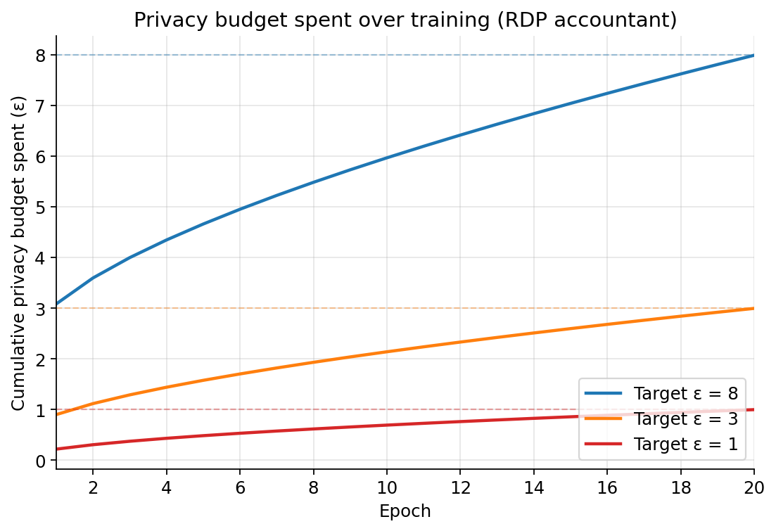
returns the privacy budget consumed so far. Logging this per epoch is how you build the $\varepsilon$-over-time chart further down.

Results

Training was done on a laptop CPU. Each run was 20 epochs. The baseline took about 23 minutes; each DP run took roughly 2 hours. The per-epoch slowdown is real and comes from the per-example gradients, not the noise.

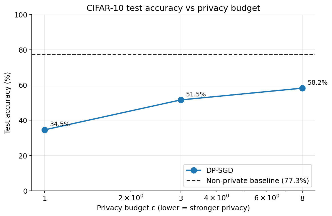
Run	Target $\varepsilon$	Final $\varepsilon$	$\sigma$	Best test acc	Final test acc
Baseline	—	—	0	77.32%	77.17%
DP	8.0	7.99	0.6461	58.18%	56.93%
DP	3.0	3.00	0.9375	51.52%	48.71%
DP	1.0	1.00	1.8750	34.54%	29.99%

The accountant hits its target almost exactly in every run, which is what you want to see. A privacy guarantee you can't verify isn't a guarantee at all.

What the numbers actually say

Below are a few observations from the data.

The first chunk of privacy is the expensive one. Going from no DP to $\varepsilon = 8$ cost 19 points of accuracy (77 to 58). Going from $\varepsilon = 8$ to $\varepsilon = 3$ cost only 7 more (58 to 51). Going from $\varepsilon = 3$ to $\varepsilon = 1$ cost 17 (51 to 34). The cost is non-linear in $\varepsilon$, and not in a monotonic way: there's a middle range where you can buy meaningful privacy for a modest utility hit, with steeper costs on either side.

$\sigma$ doesn't scale linearly with $\varepsilon$ either. $\sigma$ at $\varepsilon = 1$ is 1.875; at $\varepsilon = 8$ it's 0.646. That's about 3x more noise for 8x tighter privacy. This is the moments accountant doing real work. Under naive composition you'd need much more noise to hit $\varepsilon = 1$. The privacy amplification from Poisson subsampling and the $\sqrt{T}$ scaling of the modern accountant is what makes the lower end of the table reachable at all.

The privacy-budget chart below shows the accountant in action. Each curve grows sublinearly in epochs, which is the moments accountant's $\sqrt{T}$-style scaling in practice. At $\varepsilon = 8$ the budget is mostly spent by epoch 20; at $\varepsilon = 1$ the same training schedule eats the budget in the first few epochs and the last 15 are essentially squeezing out diminishing returns.

DP-SGD is a regularizer. The baseline overfits hard: training loss drops to 0.035 by epoch 20 while test accuracy plateaus around 77%. The DP runs barely overfit at all. Training loss stays high (1.7+ for $\varepsilon = 8$, 1.9 for $\varepsilon = 3$, 2.2 for $\varepsilon = 1$), but the train-test gap is much smaller. Clipping and noise prevent the model from memorizing individual examples, which is what privacy is supposed to do, and which incidentally also means the model can't overfit. You could read this either way: as a benefit (DP gives you free regularization) or as a caution (DP-SGD's regularization is happening whether you want it or not). Both readings are correct.

Tight privacy looks like a random walk. At $\varepsilon = 1$, accuracy oscillates between 27% and 35% across epochs with no clear convergence. With $\sigma = 1.875$, the per-step noise is overwhelming most of the signal, and the model is doing a noisy random walk that's only weakly biased toward better parameters. You can see this in the per-epoch numbers more clearly than in any summary statistic: epoch 13 dips to 26.6%, epoch 14 jumps to 33.7%, epoch 18 drops to 27.9%, epoch 19 goes back to 33.4%. This is what very tight DP-SGD looks like when the noise floor is high relative to the gradient signal. The "best test acc" column in the table above is a more honest summary of the model's actual quality than "final test acc" for this run.

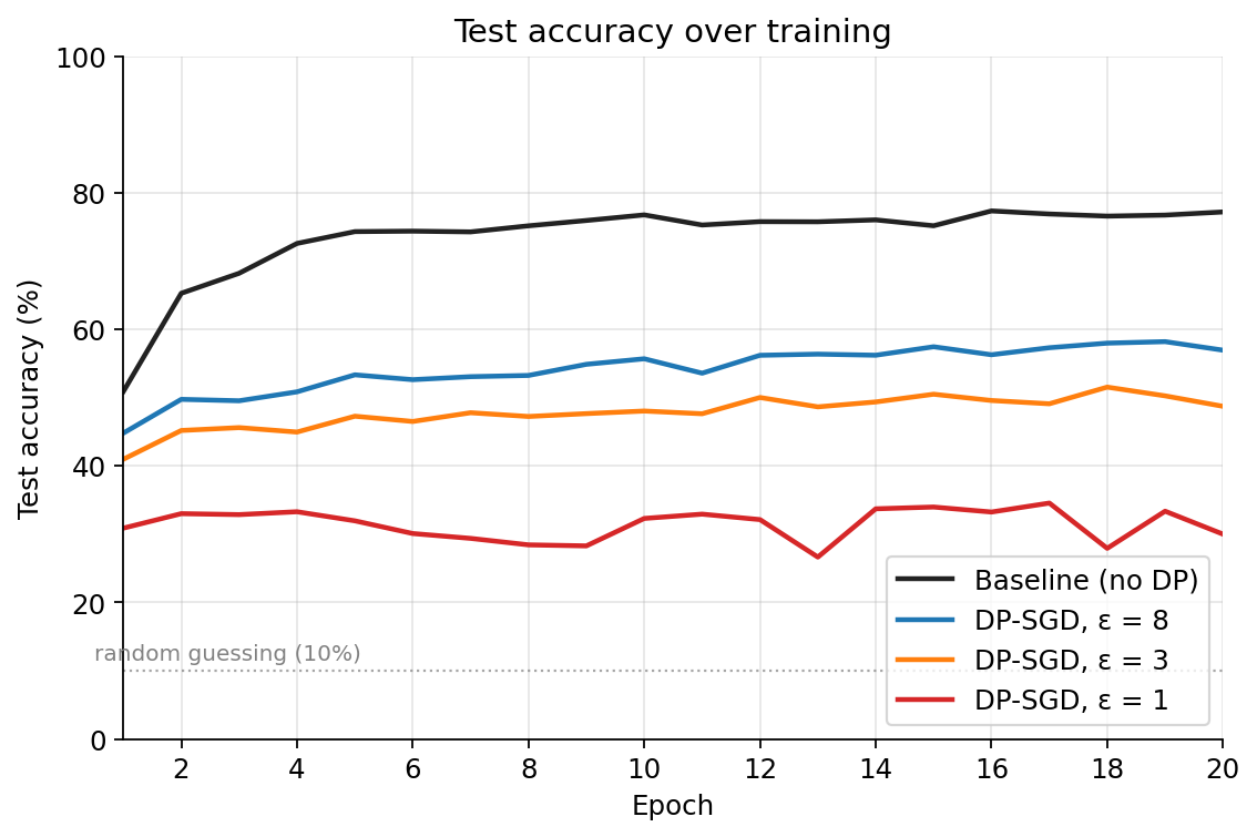
The baseline climbs fast and plateaus high; each DP run climbs more slowly to a lower plateau, with the $\varepsilon = 1$ curve barely above the chance line.

Training time is dominated by per-example gradients, not noise. All three DP runs took roughly the same wall-clock time despite very different noise multipliers. The cost of computing one gradient per example (rather than one per batch) is the bottleneck, and that cost is independent of $\sigma$. This is also why DP-SGD scales poorly to very large models: per-example gradients have to be stored separately during the backward pass.

What this experiment doesn't show

The hyperparameters here are reasonable defaults but not tuned. With careful work on the clipping norm, the learning rate schedule, longer training, and bigger batches, the DP numbers would improve, probably by several points at each $\varepsilon$. The tuning recipe from earlier in this article would be the place to start.

CIFAR-10 with a small CNN is a hard regime for DP. The dataset is small (50,000 examples is not a lot for DP, where $1/n$ scaling matters), the model is small, and there's no pretraining. The deployed systems above (VaultGemma, federated learning at Google) use either much larger datasets, pretraining on public data, or both. The accuracy gap shrinks dramatically when you have either. If you read these numbers as "DP costs 20-40 points of accuracy in general," that's wrong. It costs 20-40 points here, with these specific choices, on this specific problem. The real lesson is that DP's overhead depends heavily on scale and starting conditions.

Conclusion

DP-SGD is the algorithm that closes the loop between the theory in Part 1 and the systems that actually ship. The construction is short: per-example gradients, clipping, Gaussian noise, an accountant tracking the budget across rounds. Each piece is simple on its own, and Opacus or any other modern DP library makes wiring them together a matter of a few lines of code.

What the experiments above show is that the construction working is not the same thing as the construction being cheap. Privacy at $\varepsilon = 8$ cost us 20 points of test accuracy on CIFAR-10. Privacy at $\varepsilon = 1$ cost almost 45. But it’s also the price under the worst possible conditions for DP: small dataset, small model, no pretraining, no hyperparameter tuning. The deployed systems we looked at, VaultGemma in particular, are catching up to non-private models at the same compute, which is the direction the field has been moving for the last few years.

The math is the easy part. Picking the right unit of privacy, the right trust model, the right $\varepsilon$, the right clipping norm, the right batch size, and verifying that what your code actually does matches what your privacy analysis assumes - that’s the hard part. DP-SGD makes the math work. The rest is on you.