
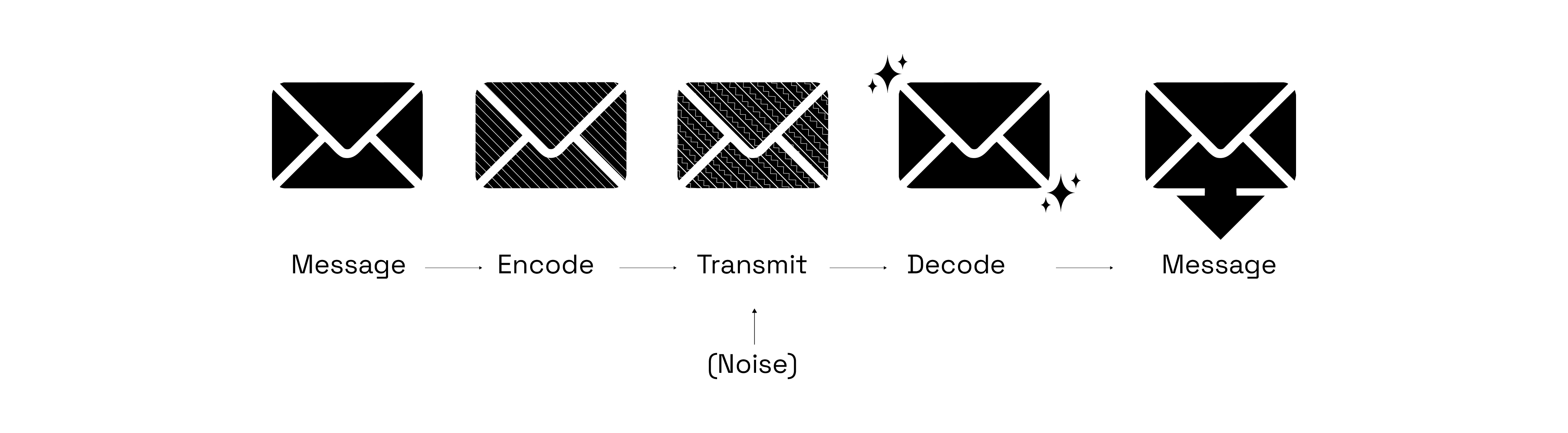
Zero Knowledge
Oct 2, 2025
A Comparison of zkVM DSLs: Halo2, Zirgen, and Plonky3
Deep dive into ZK constraint systems: Halo2's PLONKish circuits, Zirgen's STARK compiler, and Plonky3's direct AIR authoring. Complete with ...
Zero Knowledge
Sep 8, 2025

The Ethereum Foundation has announced an ambitious cryptography bounty: up to million for resolving the up-to-capacity proximity gaps conjecture for Reed–Solomon codes, specifically its strengthened variant known as mutual correlated agreement.
This might sound like an esoteric question buried deep in coding theory, but the stakes couldn't be higher. This mathematical conjecture forms the bedrock of modern zero-knowledge proofs, particularly in FRI and WHIR used in hash-based SNARKs. These proof systems are essential to Ethereum's scaling roadmap, enabling succinct and verifiable computation at massive scale.
The resolution of this conjecture will have profound implications for the entire blockchain ecosystem. If the conjecture is proven true, it would cement the security and efficiency assumptions already built into Ethereum's zk-rollup ecosystem, ensuring that current proof sizes and computational costs remain viable for years to come. However, if the conjecture is disproven, the consequences could be severe. It might invalidate current efficiency claims, forcing proof sizes to grow significantly, increasing verification times, and potentially requiring entire classes of zero-knowledge protocols to be completely redesigned.
This exploration takes you through the conjecture itself, examines our current understanding, explains its cryptographic significance, and reveals why Ethereum is willing to put serious money on the table to see this mathematical puzzle finally resolved.
To understand why this conjecture matters, we need to start with the fundamentals of error-correcting codes. An linear code represents a sophisticated mathematical structure: it's a -dimensional linear subspace within the vector space , designed with a minimum distance of between any two codewords.
Let's break down what each parameter means. The block length tells us the total length of each codeword after encoding. Think of this as how much data you actually transmit, including both the original message and the redundant information needed for error correction.
The dimension represents the number of original message symbols you want to encode. Since forms a -dimensional subspace over the finite field , it contains exactly unique codewords. The ratio gives us the rate of the code, which measures the efficiency of our encoding: how much of the transmitted data carries useful information versus redundancy.
The minimum distance determines the error-correcting power of our code. To understand this, we first need to consider the Hamming distance between two codewords and in . This distance simply counts the number of coordinate positions where the two codewords differ. The absolute minimum distance of a code is then
and we often work with the relative minimum distance
For linear codes, we denote this minimum distance by .
Finally, represents the size of our finite field, essentially determining our alphabet. Larger fields give us more flexibility but also increase computational complexity.
Reed–Solomon codes work through an elegant mathematical principle. We start with a collection of distinct points from our finite field , where typically to ensure we have enough distinct evaluation points.
The encoding process transforms a message into a polynomial. We take our message and represent it as coefficients of a polynomial of degree less than . Then we evaluate this polynomial at our chosen points, creating values. This evaluation process is the heart of Reed–Solomon encoding: we're essentially oversampling our polynomial by evaluating it at more points than strictly necessary to determine it uniquely.
This oversampling creates built-in redundancy. Even if some of these evaluation points get corrupted during transmission, we can still reconstruct the original polynomial (and hence recover our message) as long as we don't lose too many values.
Pick a message polynomial of degree , say
Evaluate on :
This vector is the codeword.
In coding theory, there's a fundamental trade-off between how efficiently we can encode information and how many errors we can correct. This trade-off is captured by the Singleton bound, which states that for any code, the minimum distance must satisfy
We can understand this bound through a clever argument called puncturing. Imagine we have a code with minimum distance , meaning any two distinct codewords differ in at least positions. Now consider what happens if we delete the first coordinates from every codeword, creating a puncturing map that takes -coordinate vectors and produces -coordinate vectors.
The key insight is that this puncturing operation remains injective when restricted to our code. If two original codewords and were different, they differed in at least positions. After deleting only coordinates, at least one differing position must remain, so . This means the punctured code has the same number of codewords as the original code .
But the punctured codewords now have length , and there are only possible vectors of this length over . Since , we must have . For a linear code with , this gives us , which rearranges to the Singleton bound:
The intuition behind this bound is elegant. Because any two codewords differ in at least places, you can erase up to coordinates and the codewords remain distinguishable. Only if you erase or more coordinates could different codewords become indistinguishable. This captures the fundamental tension between information rate and error-correcting capability.
Reed–Solomon codes meet the Singleton bound with equality, giving
This makes them Maximum Distance Separable (MDS) codes, representing the optimal balance between information rate and error correction capability. You literally cannot do better than Reed–Solomon codes in terms of this fundamental trade-off.
This optimality is why Reed–Solomon codes appear everywhere in practice, from CD players to satellite communications to modern cryptographic protocols. They squeeze the maximum error-correcting power out of every bit of redundancy, making them incredibly efficient for protecting data against corruption.
When we receive a potentially corrupted word, we need to determine whether it could plausibly have originated from our code. This requires introducing precise terminology for measuring how "close" a received word is to our code.
For any fixed error fraction , we can classify received words into two categories based on their proximity to the nearest codeword.
A received word is -close to code when there exists at least one codeword satisfying
In this case, our list of candidates is non-empty, we have at least one plausible explanation for the received word.
Conversely, a received word is -far from when every codeword satisfies
Here, our candidate list is empty; no codeword lies within our acceptable error radius.
This terminology allows us to pose the essential geometric question cleanly: given a received word and error tolerance , is close to our code or far from it?
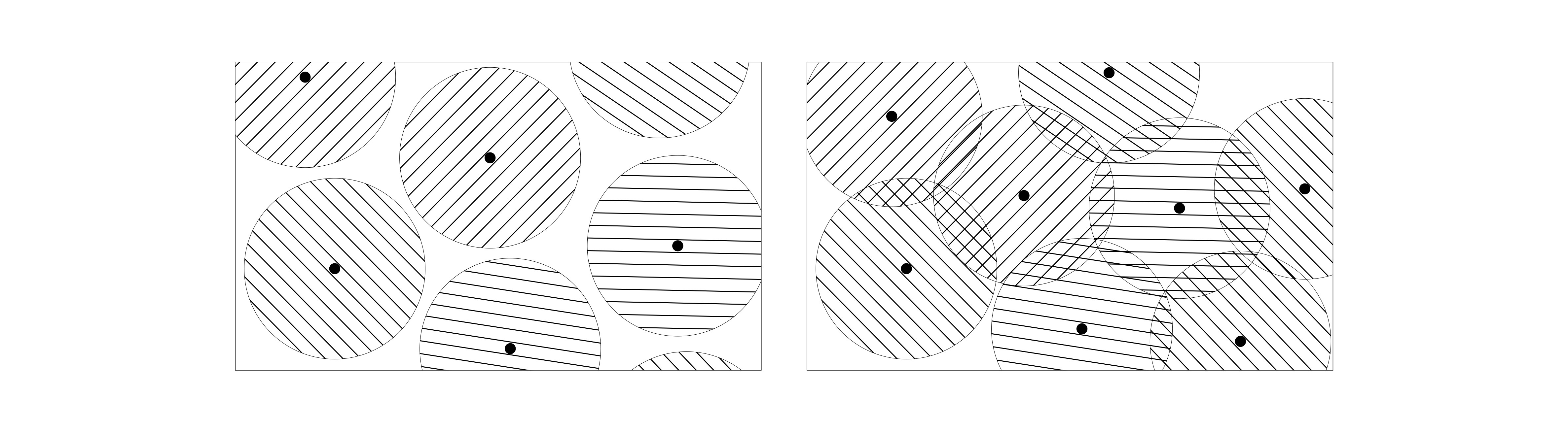
Because the minimum distance between any two distinct codewords is , their protective bubbles can have a radius of up to (but not including) before they risk touching or overlapping. This critical value defines the code’s error‑correction limit.
The maximum number of errors that a code is guaranteed to correct is denoted by and equals
Any received word with or fewer errors will always be closer to the original codeword than to any other. This is often called the unique decoding radius of the code.
Geometric intuition. Think of radius- Hamming balls around each codeword. These balls are disjoint because centers are at distance at least . Any inside a ball is uniquely decoded to that ball’s center; points outside every ball are ambiguous.
Capacity note. Pushing error tolerance toward corresponds to approaching the Singleton bound : with larger (more redundancy), the guaranteed unique-decoding radius increases; with higher rate , it decreases. This is the fundamental rate–distance trade‑off.
Traditional unique decoding demands certainty, it insists on producing exactly one unambiguous answer. When faced with ambiguity, it simply fails, leaving us with no useful information. List decoding takes a more pragmatic stance by asking a fundamentally different question: instead of desperately seeking the one true codeword, why not provide a short list of plausible candidates?
This approach transforms our decoding problem into something more manageable. Given a received word , we aim to produce all codewords that lie within some prescribed distance. The beauty of this approach lies not just in its flexibility, but in its ability to remain useful even when perfect certainty is impossible.
The critical question that emerges is obvious yet profound: how large might this list of candidates become? If the list could grow arbitrarily large, our promise of providing a manageable set of options would become meaningless. This concern brings us to one of the most important theoretical results in coding theory: the Johnson bound.
The Johnson bound provides a universal safety net, guaranteeing that under certain conditions, our list of candidates will remain small and manageable. To understand this result, we need to think in terms of relative parameters, which give us a cleaner perspective on the fundamental trade-offs involved.
Consider the relative minimum distance
which tells us about the inherent error-correcting capability of our code. We also define the relative decoding radius
representing the fraction of symbol positions where we're willing to tolerate errors.
The Johnson bound states something remarkable: for any code with relative minimum distance , and for any received word , the number of codewords lying within relative distance remains bounded by a polynomial in , provided that
This condition defines what we call the Johnson radius. Within this radius, our candidate list stays small and manageable, polynomial in size. What makes this result particularly powerful is its universality: the bound depends only on the fundamental parameters and , not on the specific structure of the code.
For Reed–Solomon codes over large fields, sophisticated algorithms like Guruswami–Sudan can achieve list decoding right up to this Johnson radius. Since Reed–Solomon codes have where is the rate, the Johnson radius becomes
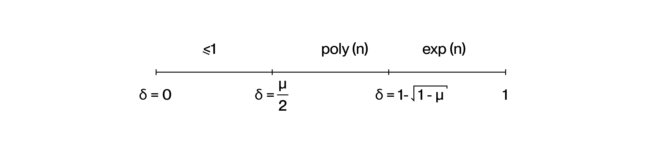
The landscape of decoding naturally divides into three distinct regimes, each characterized by the fraction of errors we're trying to handle.
The Safe Zone of Unique Decoding occurs when
Here, we remain in the comfortable world where at most one codeword can lie within our decoding radius of any received word. This is the traditional domain of classical error correction, where algorithms are simple and answers are unambiguous.
The Realm of List Decoding emerges when
We've left the safe zone of uniqueness behind, but we haven't entered chaos. The Johnson bound guarantees that our list of candidates remains small, and remarkably, efficient algorithms exist to find all candidates within this range. The Guruswami–Sudan algorithm for Reed–Solomon codes exemplifies how sophisticated mathematics can tame what initially appears to be an intractable problem.
The Combinatorial Wilderness begins when
Here, the number of potential candidates can explode exponentially, making decoding computationally infeasible for general codes. This regime represents the fundamental limits of what's possible with polynomial-time algorithms.
Imagine you're a verifier trying to check whether a bunch of vectors are valid codewords. Checking each one individually? That's going to be expensive. So here's a clever trick that cryptographers love: instead of testing each vector separately, ask the prover to mix them all together into a single random linear combination:
Now you only need to test this one combined vector to see if it's -close to your Reed–Solomon code. Pretty neat optimization, right? But here's the million-dollar question: does this shortcut actually work? If even one of the original vectors is garbage (meaning -far from the code), will the random combination still look bad with high probability?
The answer turns out to involve a beautiful mathematical phenomenon called proximity gaps.
In computer science, we love "gaps" – situations where things fall cleanly into one of two buckets with no messy middle ground. Think about classic examples like the PCP theorem (either your formula is satisfiable or it's really far from being satisfiable) or primality testing with Miller–Rabin.
Here, we're looking at the property "being a valid Reed–Solomon codeword," and we'll see this gap behavior emerge when we look at structured collections of inputs – specifically affine subspaces of .
Let's get concrete. Take a Reed–Solomon code built from polynomials of degree less than evaluated over some domain of size . Now consider a collection of subsets of – typically affine subspaces like lines or planes.
We say has a -proximity gap with respect to if every subset in behaves in one of two extreme ways:
The smaller gets, the sharper this all-or-nothing behavior becomes.
Here's the main result that makes all this practical. For Reed–Solomon codes with rate , we get proximity gaps for error fractions up to the famous Johnson radius . The collection of all affine subspaces exhibits a -proximity gap, where depends on which regime we're in:
Why should you care? This completely justifies that random linear combination trick I mentioned earlier. Pick random coefficients and form . If any of your input vectors is -far from the code, then with probability at least , your combination will also be -far. One test catches everything!
About that range: The maximum isn't arbitrary – it's exactly the Johnson/Guruswami–Sudan list-decoding radius. Some suspect the gap phenomenon might extend even further (maybe all the way to the capacity bound ), but that's still conjecture.
Field size matters: For the Johnson regime to work cleanly, you need to be roughly quadratic in (think ). But for the unique-decoding regime, is plenty.
These bounds are tight: Especially in the unique-decoding case, that bound is essentially as good as it gets. There really do exist affine lines that don't give you anything stronger.
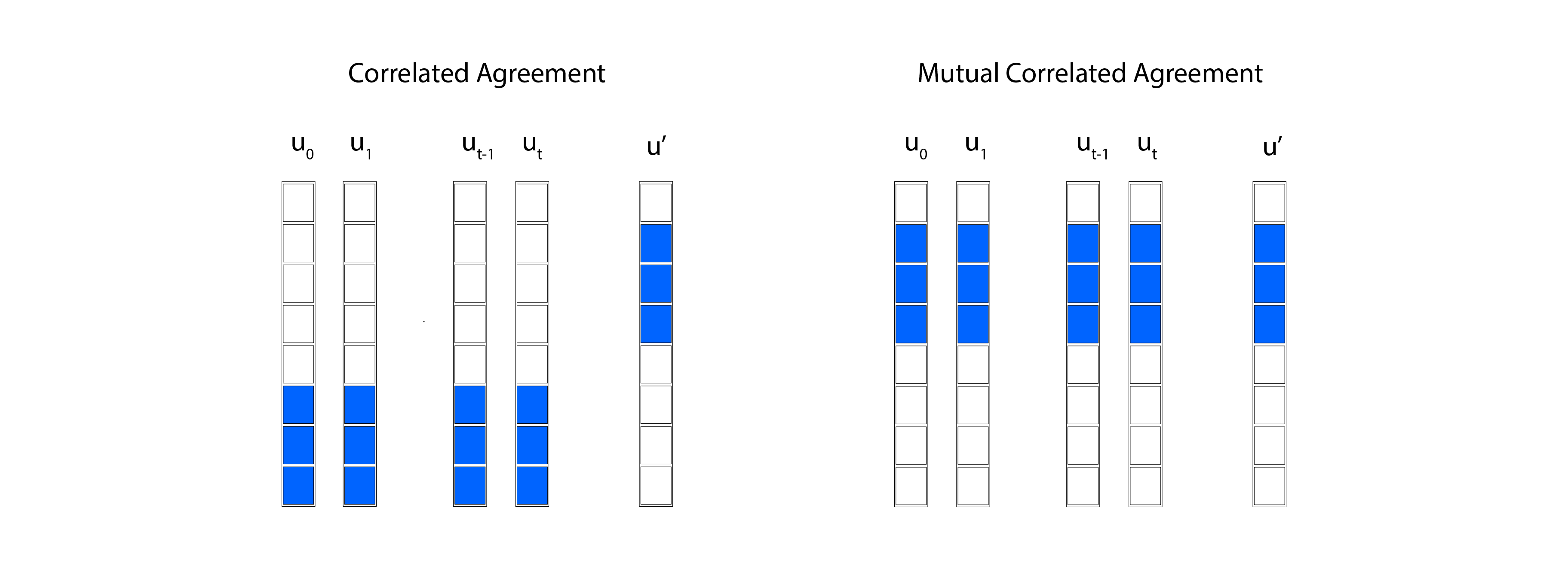
Here's a fascinating insight: suppose you take two vectors and form lots of random linear combinations, and many of those combinations happen to look close to your Reed–Solomon code. This closeness can't just be due to lucky cancellations of errors – there must be some deep structure at play. Specifically, there must be a large set of coordinates where both original vectors already agree with some codewords from your code. This shared structure is what we call correlated agreement.
Let's work with our Reed–Solomon code over evaluation domain . I'll think of codewords as functions on , so . We'll use for Hamming distance and write for the distance from to the nearest codeword.
Fix your proximity parameter and that error parameter from the proximity gap theorem we just discussed.
Take two vectors and look at the affine line they generate:
Now suppose a significant fraction of points on this line are -close to the code:
Then something remarkable happens: there must exist a large subdomain and actual codewords such that:
In plain English: if many combinations look close to your code, it's because and each agree with some codeword on a common large fraction of coordinates.
This extends naturally to higher-dimensional affine spaces. Take vectors and consider:
If enough points in are close to the code (more than that fraction), then there's a large coordinate set where all the generators simultaneously agree with corresponding codewords .
Correlated agreement gives us a sufficient condition for those proximity gaps we want. Intuitively, if a batch of linear combinations often looks close to the code, that's only possible when all the underlying vectors share a large "agreement region" with the code.
The big open question? We don't know if correlated agreement is also necessary for proximity gaps. Maybe there are other ways to get gaps that work beyond the Johnson radius (for ) without going through this agreement structure.
Once you have correlated agreement, the proximity gap theorem becomes almost obvious. Every line falls into one of two categories:
Here's where things get really interesting for modern cryptographic protocols. Systems like WHIR don't just check a single random linear combination per round. They create several different mixtures of the same base vectors – think folding operations, shifts, different combination patterns. To maintain tight soundness when you're batching all these checks together, you need something stronger than ordinary correlated agreement.
You need the same large coordinate set to witness agreement simultaneously across your entire family of mixture operations. This is Mutual Correlated Agreement (MCA).
Let be your family of affine-linear mixture operations that your verifier uses in a given round. For each operation , suppose you have:
for some reasonable measure over the mixing parameters .
The mutual correlated agreement conjecture says there should exist a single coordinate set with and a consistent family of codewords such that simultaneously for all and all parameters :
The key word is "mutual" – one common "good" coordinate set that works for your entire mixture family, not separate sets for each operation.
Proved for unique-decoding: The WHIR paper establishes MCA when , which enables their "no soundness degradation" result when batching multiple checks per round.
The big conjecture: Extending MCA to the Johnson regime () or even further ("up to capacity" at ) is now one of the central open problems in the field.
Why it matters: A proof would give us the tightest possible soundness analysis for the fastest transparent Reed–Solomon-based protocols. A counterexample would force us to redesign parameters or protocols.
The Ethereum Foundation's million-dollar bounty represents more than just a mathematical challenge, it's a strategic investment in the cryptographic foundations of scalable blockchain infrastructure. The mutual correlated agreement conjecture for Reed-Solomon codes sits at the intersection of pure mathematics and practical cryptography, where theoretical breakthroughs directly translate into real-world impact.
Our exploration reveals why this particular conjecture matters so much. Reed-Solomon codes already provide the optimal trade-off between information rate and error correction (achieving the Singleton bound), making them the natural choice for cryptographic protocols. The proximity gap phenomenon allows efficient batch verification of multiple statements simultaneously, dramatically reducing the computational overhead of zero-knowledge proofs. But to push these efficiencies to their theoretical limits, especially in protocols like WHIR that perform complex mixture operations, we need the stronger guarantee provided by mutual correlated agreement.
The stakes are clear. A positive resolution would validate the security assumptions underlying Ethereum's scaling roadmap, confirming that current zk-rollup architectures can maintain their efficiency guarantees as they scale to global adoption. The mathematical proof would demonstrate that batched verification techniques can be pushed right up to the Johnson radius (or potentially even the capacity bound) without sacrificing soundness.
Conversely, a negative result would force a fundamental reassessment of how we design transparent zero-knowledge protocols. Proof sizes might need to grow, verification times could increase, and entire classes of optimizations might prove unsound. The cryptographic community would need to develop new approaches that work within whatever limitations a counterexample reveals.
This exploration builds upon the foundational work of countless researchers in coding theory, cryptography, and complexity theory. The theoretical foundations of proximity gaps for Reed-Solomon codes are comprehensively treated in "Proximity Gaps for Reed–Solomon Codes", which established many of the fundamental results discussed in our exploration of the Johnson radius and correlated agreement phenomena. The practical cryptographic applications and the mutual correlated agreement conjecture are detailed in "WHIR: Reed–Solomon Proximity Testing with Super-Fast Verification", whose authors identified this mathematical bottleneck as crucial for achieving optimal soundness in batched verification protocols. We are particularly grateful to Thomas Coratger from the Ethereum Foundation for his ongoing work in this area, including his comprehensive repository on proximity proofs which provides valuable pedagogical materials that helped inform our exposition.

