Zero Knowledge in STARKs

STARKs are one of the most exciting proof systems in the cryptography space today. They're transparent, scalable, post-quantum secure, and deeply mathematical. But one aspect of STARKs that can feel underexplained is how zero-knowledge is actually achieved. This blog post is here to fix that.

We dive into the elegant techniques behind zero-knowledge in STARKs. We'll learn why just adding randomness isn't enough and why the DEEP composition polynomial needs special attention.

Whether you're building a STARK prover or just trying to understand what happens under the hood, this post aims to give you the clearest and most accurate breakdown of how zero-knowledge is implemented in practice.

Notation

Before we get into the mechanics, let's define some recurring notation and parameters:

• $\mathbb{F}$ — Finite field of size $p$; $\mathbb{F}^*$ multiplicative subgroup of $\mathbb{F}$.
• $\mathbb{K}$ — Extension field of degree $e$, $|\mathbb{K}| = p^e$.
• $\mathbb{G}$ — Cyclic subgroup of $\mathbb{F}^*$ with generator $g$, $|\mathbb{G}| = n$.
• $\mathbb{H}$ — Coset of a cyclic subgroup of $\mathbb{F}^*$, $|\mathbb{H}| = m, m > n$.
• $Z_G(X) = X^n - 1$ — vanishing polynomial of $\mathbb{G}$.

Overview

STARKs (Scalable Transparent ARguments of Knowledge) are cryptographic proof systems that allow a prover to convince a verifier that a certain computation was performed correctly, without revealing the computation's internal details or requiring the verifier to re-execute it. They are particularly attractive due to their transparency (no trusted setup) and post-quantum security.

At their core, STARKs reduce computational integrity to statements about polynomials over finite fields. The prover constructs a low-degree polynomial encoding the execution trace of a computation, commits to it using a Merkle tree, and then proves its validity through algebraic checks and interactive proofs. The verifier only needs to inspect a few values and Merkle paths to be convinced with high confidence.

A typical STARK proof involves the following steps:

• Trace Generation — Evaluate the state of the computation at each step and record it in a trace table.

  $$\vec{r}_i = \left[r_i^{(0)}, r_i^{(1)}, \dots, r_i^{(k-1)}\right] \in \mathbb{F}^k$$

• Polynomial Interpolation — Represent trace columns as low-degree polynomials.

  $$T_j(X) \in \mathbb{F}[X], \quad \deg(T_j) < n$$

• The Quotient Polynomial — Define transition and boundary constraints using polynomial identities.

  $$$$

• Low-Degree Extension (LDE) — Extend trace and quotient polynomials to a larger evaluation domain to enable probabilistic low-degree testing.

  $$T_j(x),\quad Q(x) \quad \text{evaluated at } x \in \mathbb{H}$$

• Commitment — Hash LDE evaluations into a Merkle tree to create a succinct commitment.

$$\text{Commit}\left(T_j|_{\mathbb{H}}\right),\quad \text{Commit}\left(Q|_{\mathbb{H}}\right)$$

• Trace Consistency Check — Perform evaluations outside the original domain to strengthen soundness by checking that the quotient polynomial is consistent with the constraints over the trace polynomials. Evaluate

  $$T_j(z),\quad Q(z) \quad \text{for random } z \in \mathbb{K} \setminus (\mathbb{H} \cup \mathbb{G})$$

  and check that

  $$Q(z) = \sum_i \epsilon_i \cdot \frac{C_i(T_1(z), ..., T_k(z), T_1(gz), ..., T_k(gz))}{Z_i(z)}$$

  where $Z_i(X)$ is a vanishing polynomial over the constraint domain.

• FRI Protocol — Prove that the DEEP composition polynomial has low degree.

  $$\begin{aligned} F(X) = \sum_i \alpha_i \cdot \frac{T_i(X) - T_i(z)}{X - z} + \sum_i \beta_i \cdot \frac{T_i(gX) - T_i(gz)}{X - gz} \\ + \sum_i \gamma_i \cdot \frac{Q_i(X) - Q_i(z^S)}{X - z^S} \end{aligned}$$

  where $Q(X) = \sum_{i=1}^{S} \lambda^{i-1} \cdot Q_i(X^S)$

• Verification — The verifier checks a small number of evaluations and Merkle paths to validate the proof.

Adding Zero Knowledge

Soundness ensures that false claims are rejected with high probability — but it doesn't prevent the verifier from learning something unintended about the prover’s witness. For full privacy, we want zero knowledge: the verifier should learn nothing about the internal computation beyond the fact that it was carried out correctly.

This is subtle in the context of STARKs. Even though no part of the witness is revealed directly, certain components — like evaluations in the Low-Degree Extension (LDE) domain, or out-of-domain (DEEP) queries — can unintentionally leak information.

To address this, modern STARK systems incorporate two distinct layers of masking:

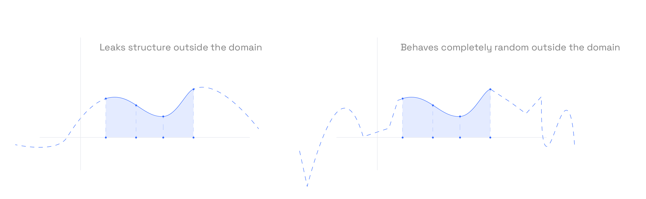
• Witness Masking — Before committing to the trace polynomials, the prover adds a random low-degree polynomial (drawn independently for each column) to each trace polynomial. These masks are chosen to vanish on the original evaluation domain $\mathbb{G}$, ensuring they don’t affect constraint satisfaction. But outside $\mathbb{G}$ — especially on the larger evaluation domain $\mathbb{H}$ used for the LDE — they act as effective noise, hiding the true values.

• DEEP composition polynomial Masking — Even after masking the witness, the constraint system can leak information through the DEEP composition polynomial. Since this polynomial encodes evaluations over $\mathbb{H}$, and the verifier queries it at random points, it must also be masked. The prover adds a random low-degree polynomial to the final DEEP composition polynomial. Care must be taken to ensure that this additive mask maintains the degree bounds required for soundness and zero knowledge.

In summary: adding randomness alone isn’t enough — it must be structured randomness, carefully aligned with the algebraic structure of the proof system. Masking both the trace and the DEEP composition polynomial is essential for turning a sound STARK into a zero-knowledge STARK.

Masking the Witness Polynomials

The verifier interacts with the trace polynomials in two key ways: during the FRI phase, which tests their low-degree structure over the evaluation domain, and during the trace consistency check, which evaluates constraint expressions at random points outside the evaluation domain. Both of these can potentially leak information about the execution trace.

To achieve zero knowledge, we mask each trace column polynomial by adding structured randomness that hides its values outside the original trace domain, while preserving correctness within it. This is done by multiplying a random low-degree polynomial with the vanishing polynomial of the trace domain.

Let $T_i(X) \in \mathbb{F}[X]^{<n}$ denote the $i$th trace polynomial interpolated over a domain $\mathbb{G} \subset \mathbb{F^*}$. The masked version is defined as:

$$\hat{T}_i(X) = T_i(X) + Z_{\mathbb{G}}(X) \cdot R_i(X), \quad \text{where } Z_{\mathbb{G}}(X) = \prod_{g \in \mathbb{G}} (X - g),$$

and $R_i(X) \leftarrow \mathbb{F}[X]^{<h}$ is a random masking polynomial of degree less than $h$.

This masking ensures the following:

• Correctness over the trace domain: For any $x \in \mathbb{G}$, we have $Z_{\mathbb{G}}(x) = 0$, so the masked polynomial agrees with the original:

  $$\hat{T}_i(x) = T_i(x) \quad \forall\, x \in \mathbb{G}.$$

  Thus, all transition and boundary constraints remain satisfied over the trace domain.

• Randomness outside the domain: For any $z \notin \mathbb{G}$, the vanishing polynomial satisfies $Z_{\mathbb{G}}(z) \ne 0$, so:

$$\hat{T}_i(z) = T_i(z) + Z_{\mathbb{G}}(z) \cdot R_i(z),$$

which is uniformly random in $\mathbb{F}$, provided $R_i$ is drawn uniformly. This ensures that the masked trace reveals nothing about the original trace at any queried point outside $\mathbb{G}$.

• Query privacy: Since all FRI queries and trace consistency checks occur at points outside $\mathbb{G}$, each such evaluation of $\hat{T}_i$ appears statistically independent of the original $T_i$, protecting the witness from leakage.

Masking the DEEP Composition Polynomial

Even after masking the witness polynomials, zero-knowledge is not guaranteed. The issue arises during the FRI protocol, where the DEEP composition polynomial $F(X)$ is tested for low degree. In this process, the verifier repeatedly folds $F(X)$ to reduce its degree — and with each fold, some randomness from the original masking polynomials is also folded and lost.

A Note on Splitting the Quotient Polynomial

Before applying the FRI protocol, the quotient polynomial $Q(X)$ must be brought into a form suitable for low-degree testing. Specifically, we require all polynomials passed to FRI to have degree of some power of two, which allows efficient recursive folding.

We begin by multiplying $Q(X)$ by an appropriate factor to increase its degree to the next power of two:

$$\deg(Q) < D, \quad \text{where } D = 2^{\lceil \log_2(\deg(Q)) \rceil}.$$

We then split $Q(X)$ into $S = D / n$ parts, where $n = |\mathbb{G}|$ is the size of the trace domain. This ensures that each component has degree strictly less than $n$, so that it can be committed and checked individually by FRI.

The decomposition is written as:

$$Q(X) = \sum_{j=0}^{S-1} X^j \cdot Q_j(X^S), \quad \text{with each } Q_j(X) \in \mathbb{F}[X]^{<n}.$$

This structure allows the verifier to check all $Q_j$ in parallel, using a single low-degree protocol with $\deg(Q_j) < n$, and supports efficient Merkle tree commitments and folding.

After splitting $Q(X)$ into $S$ components $Q_j(X)$, the prover then constructs the DEEP composition polynomial $F(X)$, which checks that:

• $T_i(X)$ agrees with its claimed value at $z$,
• $T_i(gX)$ agrees with its value at $g z$,
• Each quotient component $Q_j(X)$ agrees with its value at $z^S$.

This gives the final expression:

$$\begin{aligned} F(X) = \sum_i \alpha_i \cdot \frac{T_i(X) - T_i(z)}{X - z} \,+\, \sum_i \beta_i \cdot \frac{T_i(gX) - T_i(gz)}{X - gz} \,+\, \sum_j \gamma_j \cdot \frac{Q_j(X) - Q_j(z^S)}{X - z^S} \end{aligned}$$

where the $\alpha_i, \beta_i, \gamma_j \in \mathbb{F}$ are verifier-chosen randomizers to bind the prover to all constraint evaluations simultaneously.

This polynomial $F(X)$ is now subject to a low-degree check via FRI, and its correctness implies that all DEEP queries were answered consistently — across both the trace and the quotient parts.

Why masking the DEEP composition polynomial is necessary

Each trace polynomial $T_i(X)$ is masked by a polynomial of the form $Z_{\mathbb{G}}(X) \cdot R_i(X)$, and the DEEP composition polynomial $F(X)$ is computed from these masked traces. This means the randomness from $R_i(X)$ is already embedded in $F(X)$.

However, FRI recursively folds $F(X)$ — and in each fold, the degree is halved. Crucially, this also halves the effective entropy of the randomness inside $F(X)$. After several rounds, very little randomness remains, and the verifier may begin to observe statistical biases correlated with the underlying witness.

To prevent this leakage, we add fresh randomness directly to the polynomial before the FRI protocol begins.

Adding entropy via masking

Let $|\mathbb{G}| = n$ be the size of the trace domain, and let $h$ be the masking degree used for the witness polynomials. We define the final quotient DEEP composition polynomial as:

$$H(X) = F(X) + R(X),$$

where $R(X) \leftarrow \mathbb{F}[X]^{<n + h - 1}$ is a uniformly random masking polynomial of sufficiently high degree.

This fresh term $R(X)$ does not affect any constraint checks (since FRI only verifies low-degree structure), but it ensures that the folded evaluations of $H(X)$ remain statistically indistinguishable from random — even after multiple rounds of degree halving.

Choosing the masking degree $h$

The degree of $R(X)$ must be high enough to ensure that the prover’s responses remain statistically hidden even after many FRI rounds and trace consistency checks.

Let’s carefully account for the total number of degrees of freedom that could be leaked:

• Trace consistency queries: Each check at a point $z \in \mathbb{K}$ (an extension field of degree $e$) reveals $e$ independent scalars over $\mathbb{F}$. The number of such queries is $n_D$.
• Shifted constraints: For each query, the verifier evaluates both $\hat{T}_i(z)$ and $\hat{T}_i(gz)$, effectively doubling the leakage. This introduces a factor of 2.
• Quotient splitting and implicit queries: After splitting $Q(X)$ into $S$ component polynomials $Q_j(X)$, each evaluation at $Q_j(z^S)$ leaks information about the values of $Q(X)$ at the $S$ points $z \cdot U$, where $U$ is the group of $S$-th roots of unity. Hence, the masking budget must scale with $S$.
• FRI-root quotient dependency: During FRI, each round operates on a domain composed of a coset of a subgroup of size $S$, meaning that evaluating any one $Q_j(X)$ at a FRI point implicitly depends on the values of $Q(X)$ at $S$ positions. Since quotient values are computed from the trace evaluations, and FRI folds over these positions recursively, the trace masking must account for $2 \cdot S \cdot n_F$ evaluations: one for each FRI query point and its $g$-shift across the $S$-root coset.
• Direct FRI spot-checks: FRI also performs $n_F$ spot-checks in its folded tables, and these are generally disjoint from the previous queries. Thus, they must be independently masked, contributing an additional $n_F$ degrees.

Therefore, to protect against all forms of leakage, the masking degree must satisfy:

$$h \;\ge\; 2 \cdot S \cdot (e \cdot n_D + n_F) \;+\; n_F.$$

Why this works

Lemma: Let $\hat{T}_1(X), \dots, \hat{T}_k(X)$ be masked trace polynomials as defined earlier, and suppose we split the quotient polynomial $Q(X)$ into $S$ components:

$$Q(X) = \sum_{j=1}^{S} X^j \cdot Q_{j}(X^S), \quad \text{with each } Q_j(X) \in \mathbb{F}[X]^{<n}.$$

Let $Q_{DEEP} \subset \mathbb{F} \setminus (\mathbb{H} \cup \mathbb{G})$ and $Q_{FRI} \subset \mathbb{H}$ be sets of DEEP and FRI query points respectively, with

$$|Q_{FRI}| \le n_F, \quad |Q_{DEEP}| \le n_D.$$

Assume the masking degree $h$ satisfies the entropy bound:

$$h \ge 2 \cdot d \cdot (e\,n_D + n_F) + n_F.$$

Then the joint distribution of all queried values:

$$\left\{ \begin{aligned} &\left( \hat{T}_1(z),\; \hat{T}_1(gz),\; \dots,\; \hat{T}_M(z),\; \hat{T}_M(gz),\; Q_1(z^d),\; \dots,\; Q_d(z^d) \right) \quad \text{for } z \in Q_{DEEP}, \\ &\left( \hat{T}_1(z),\; \dots,\; \hat{T}_M(z),\; Q_1(z),\; \dots,\; Q_d(z) \right) \quad \text{for } z \in Q_{FRI} \end{aligned} \right\}$$

is statistically independent of the original (unmasked) witness polynomials $T_1(X), \dots, T_M(X) \in \mathbb{F}[X]$.

In other words, even after observing all DEEP queries, their $g$-shifts, and FRI spot-checks on the quotient components, the verifier learns nothing about the witness values — provided the masking degree is large enough.

Toy Example

To make the abstract steps of zero-knowledge STARKs concrete, we will walk through a small, fully specified example over a finite field. This example will serve as a running reference, illustrating each part of the protocol with concrete values.

We work over the prime field:

$$\mathbb{F} = \mathbb{F}_{97}.$$

The multiplicative group $\mathbb{F}_{97}^*$ has order 96 and is cyclic. Let $g = 5 \in \mathbb{F}_{97}$ be a generator. We define two multiplicative subgroups:

• Trace domain: $\mathbb{G} = \langle g^{12} \rangle$, a subgroup of order 8,
• LDE domain: $H = \langle 21 * g^6 \rangle$, a coset of order 16

This mirrors a typical STARK setup: we interpolate the trace over $\mathbb{G}$, then extend it to $H$ for low-degree testing and constraint evaluation.

The Computation

We model a simple computation: an 8-step Fibonacci sequence, defined recursively as:

$$t_{i+2} = t_{i+1} + t_i \mod 97.$$

With initial values:

$$t_0 = 89, \quad t_1 = 90.$$

Evaluating the recurrence gives the following execution trace:

Step $i$	$t_i$
0	89
1	90
2	82
3	75
4	60
5	38
6	1
7	39

These values represent the internal state of our computation over time. In a STARK proof, we will interpolate these values into a trace polynomial over the trace domain $\mathbb{G}$, then extend it to the larger domain $\mathbb{H}$ as part of the low-degree extension (LDE) phase.

Let $T(X)$ be the unique polynomial of degree less than 8 that satisfies:

$$T(g^{12 \cdot i}) = t_i \quad \text{for } i = 0, \dots, 7.$$

Interpolating the Fibonacci values:

$$[89,\ 90,\ 82,\ 75,\ 60,\ 38,\ 1,\ 39]$$

we obtain the trace polynomial:

$$T(X) = 55X^7 + 71X^6 + 18X^5 + 23X^4 + 34X^3 + 91X^2 + 53X + 35 \in \mathbb{F}_{97}[X].$$

This polynomial encodes the entire trace over $\mathbb{G}$, and will serve as the starting point for witness masking and constraint verification in the next steps.

Masking the Trace Polynomial

To ensure zero knowledge, we mask the trace polynomial by adding a multiple of the vanishing polynomial over the trace domain $\mathbb{G}$. This preserves all values on $\mathbb{G}$, but randomizes evaluations elsewhere.

Let $Z_{\mathbb{G}}(X) = X^8 - 1$, the vanishing polynomial over $\mathbb{G}$, and let $r(X) \in \mathbb{F}_{97}[X]^{<h}$ be a random masking polynomial. For this example, we choose:

$$\begin{aligned} R(X) =\; &71X^{23} + 51X^{22} + 79X^{21} + 31X^{20} \\ &+ 22X^{19} + 45X^{18} + 3X^{17} + 30X^{16} \\ &+ 57X^{15} + 48X^{14} + 94X^{13} + 44X^{12} \\ &+ 20X^{11} + 65X^{10} + 9X^9 + 86X^8 \\ &+ 19X^6 + 37X^5 + 32X^4 + 54X^3 \\ &+ 26X^2 + 88X + 65. \end{aligned}$$

where the degree is chosen as follows: the number of FRI queries is $n_F = 3$, the number of DEEP queries is $n_D = 1$, the splitting factor for the quotient polynomial is $S = 2$. With these numbers we can calculate the lower bound for $h$ as $h > 2 * 2(2*1 + 3) + 3 = 23$.

The masked trace polynomial is:

$$\hat{T}(X) = T(X) + (X^8 - 1) \cdot R(X).$$

Substituting in the expression for $T(X)$, we get:

$$\begin{aligned} \hat{T}(X) =\; &55X^7 + 71X^6 + 18X^5 + 23X^4 + 34X^3 + 91X^2 + 53X + 35 \\ &+ (X^8 - 1)\cdot(71X^{23} + 51X^{22} + 79X^{21} + 31X^{20} \\ &\qquad + 22X^{19} + 45X^{18} + 3X^{17} + 30X^{16} + 57X^{15}\\ &\qquad + 48X^{14} + 94X^{13} + 44X^{12} + 20X^{11} + 65X^{10}\\ &\qquad + 9X^9 + 86X^8 + 19X^6 + 37X^5 + 32X^4\\ &\qquad + 54X^3 + 26X^2 + 88X + 65)\\ \end{aligned}$$

This polynomial agrees with $T(X)$ at all points in $\mathbb{G}$, but appears pseudorandom at any $z \notin \mathbb{G}$, such as those used in trace consistency checks or FRI.

Conclusion

Zero‑knowledge in STARKs rests on two complementary masks:

• Witness masking, which hides the raw execution trace outside $\mathbb{G}$.
• DEEP composition polynomial masking, which protects the polynomial used in FRI, ensuring entropy never depletes.

Together, these ensure that a STARK proof reveals nothing beyond the truth of the statement, while preserving transparency, scalability, and post‑quantum security.

Acknowledgments

This post is based on and inspired by the excellent 2024 technical note “A Note on Adding Zero-Knowledge to STARKs” by Ulrich Haböck and Al Kindi. Their paper offers a clear and rigorous treatment of witness masking, quotient decomposition, and entropy accounting in small-field STARK systems. Many of the ideas and formal guarantees discussed here — especially those involving FRI, DEEP queries, and the structure of masking polynomials — are direct adaptations or intuitive explanations of results presented in that work.